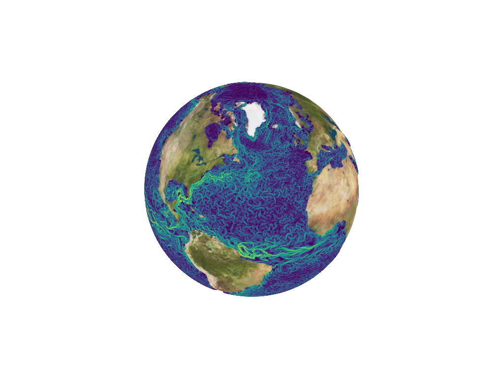
Copernicus Globe FTLE

Compute the FTLE field over the entire globe for ocean flow at time of using Copernicus reanalysis data.

# Author: ajarvis
# Data: Copernicus Marine Service - Global Ocean Physics Reanalysis
from math import copysign
import numpy as np
from numbacs.flows import get_globe_flow
from numbacs.integration import flowmap
from numbacs.diagnostics import ftle_icosphere
from numbacs.utils import (
    convert_vel_to_3D,
    icosphere_and_displacements,
    fill_nans_and_get_mask,
)

Get flow data

Load in ocean velocity data, dates, and coordinates. Set domain for FTLE computation and integration span. Create interpolant and retrieve flow.

# load in atmospheric data
dates = np.load("../data/copernicus/dates.npy")
dt = 1.0
t = np.arange(0, len(dates) * dt, dt, np.float64)
lon_rad = np.deg2rad(np.load("../data/copernicus/lon.npy")).astype(np.float64)
lat_rad = np.deg2rad(np.load("../data/copernicus/lat.npy"))
r = 6371.0
# NumbaCS uses 'ij' indexing, most geophysical data uses 'xy'
# indexing for the spatial coordintes. We need to switch axes and
# scale by 3.6 since velocity data is in m/s and we want km/hr.
u = np.moveaxis(np.load("../data/copernicus/uo_mean_coarse.npy"), 1, 2) * 86.4
v = np.moveaxis(np.load("../data/copernicus/vo_mean_coarse.npy"), 1, 2) * 86.4
nt, nx, ny = u.shape

# fill nan values in velocity fields with 0.0 and return mask
u, v, grid_mask = fill_nans_and_get_mask((u, v))

# set t0, integration span, and integration direction
day = 1
t0_date = np.datetime64(f"2020-01-{day:02d}")
kt0 = np.argwhere(dates == t0_date)[0][0]
t0 = t[kt0]
T = 45.0
params = np.array([copysign(1, T)])

# convert vel to xyz coords
vx, vy, vz = convert_vel_to_3D(u, v, lon_rad, lat_rad)

# get interpolant for particle integration on the globe, set pole to 'north'
# because only the north pole is included in velocity data
funcptr = get_globe_flow(t, lon_rad, lat_rad, vx, vy, vz, pole="north")

Create mesh on icosphere

Generate mesh on icosphere, find neighbors of each vertex, compute displacements for each neighbor, and get masks for mesh. Generally subdivides between 7 - 9 will be sufficient. 7 will be fastest but least resolved (166,382 intial conditions), 8 will be reasonably fast and resolved (655,362 initial conditions), and 9 will be slowest but most resolved (2,621,422 initial contiions).

subdivides = 8
mesh_points, neighbors, X, mask, dilated_mask = icosphere_and_displacements(
    subdivides, r=r, mask_data=(grid_mask, lon_rad, lat_rad)
)

Integrate

# lessen tolerances for scale and speed
rtol = 1e-3
atol = 1e-5

# compute flowmap for icosphere mesh, pass in mask to ignore masked points
flowmap_ico = flowmap(funcptr, t0, T, mesh_points, params, rtol=rtol, atol=atol, mask=mask)

FTLE

# compute ftle using least squares approximation, pass in dilated mask
# to ignore ftle computations at mask and mask boundaries
ftle_ico = ftle_icosphere(flowmap_ico, neighbors, X, T, mask=dilated_mask)

Plot

Note

Plotting requires pyvista and vedo to be installed. These can be installed easily with pip or conda. If run from a python script or jupyter notebook, this will generate an interactive plot, we just show a screenshot here.

# import pyvista and vedo, load earth object and create PolyData object for
# earth and icosphere with FTLE
import pyvista as pv
import vedo

# use vedo earth for plotting, rotate to match our lon data
vedo_earth = vedo.Earth(r=r).rotate_z(180)

# convert to pyvista object and extract texture
pv_earth = pv.wrap(vedo_earth.dataset)
earth_texture = vedo_earth.actor.GetTexture()

mesh = pv.PolyData(mesh_points[~dilated_mask])
mesh.point_data["ftle"] = ftle_ico[~dilated_mask]

# create plotter object, use no lighting
pl = pv.Plotter(lighting="none")

# add icosphere mesh
pl.add_mesh(mesh, scalars="ftle", render_points_as_spheres=True, show_scalar_bar=False)

# add earth mesh and texture
pl.add_mesh(pv_earth, texture=earth_texture)

# rotate camera and show plot
pl.camera.azimuth = -90
pl.show()