MERRA-2 Globe FTLE

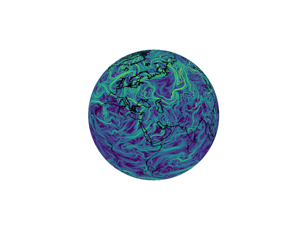
Compute the FTLE field over the entire globe for atmospheric flow at time of Godzilla dust storm using MERRA-2 data which is vertically averaged over pressure surfaces ranging from 500hPa to 800hPa.

# Author: ajarvis
# Data: MERRA-2 - Global Modeling and Assimilation Office - NASA
from math import copysign
import numpy as np
from numbacs.flows import get_globe_flow
from numbacs.integration import flowmap
from numbacs.diagnostics import ftle_icosphere
from numbacs.utils import convert_vel_to_3D, icosphere_and_displacements, lonlat2xyz

Get flow data

Load in atmospheric velocity data, dates, and coordinates. Set domain for FTLE computation and integration span. Create interpolant and retrieve flow.

# load in atmospheric data
dates = np.load("../data/merra_june2020/dates.npy")
dt = (dates[1] - dates[0]).astype("timedelta64[h]").astype(int)
t = np.arange(0, len(dates) * dt, dt, np.float64)
lon_rad = np.deg2rad(np.load("../data/merra_june2020/lon.npy"))
lat_rad = np.deg2rad(np.load("../data/merra_june2020/lat.npy"))
r = 6371.0
# NumbaCS uses 'ij' indexing, most geophysical data uses 'xy'
# indexing for the spatial coordintes. We need to switch axes and
# scale by 3.6 since velocity data is in m/s and we want km/hr.
u = np.moveaxis(np.load("../data/merra_june2020/u_500_800hPa.npy"), 1, 2) * 3.6
v = np.moveaxis(np.load("../data/merra_june2020/v_500_800hPa.npy"), 1, 2) * 3.6
nt, nx, ny = u.shape

# set t0, integration span, and integration direction
day = 16
t0_date = np.datetime64(f"2020-06-{day:02d} 00")
kt0 = np.argwhere(dates == t0_date)[0][0]
t0 = t[kt0]
T = -72.0
params = np.array([copysign(1, T)])

# convert vel to xyz coords
vx, vy, vz = convert_vel_to_3D(u, v, lon_rad, lat_rad)

# get interpolant for particle integration on the globe
funcptr = get_globe_flow(t, lon_rad, lat_rad, vx, vy, vz)

Create mesh on icosphere

Generate mesh on icosphere, find neighbors of each vertex, and compute displacements for each neighbor, Generally subdivides between 7 - 9 will be sufficient. 7 will be fastest but least accurate (166,382 intial conditions), 8 will be reasonably fast and accurate (655,362 initial conditions), and 9 will be slowest but most accurate (2,621,422 initial contiions).

subdivides = 8
mesh_points, neighbors, X = icosphere_and_displacements(subdivides, r=r)

Integrate

# lessen tolerances for scale and speed
rtol = 1e-3
atol = 1e-5

# compute flowmap for icosphere mesh
flowmap_ico = flowmap(funcptr, t0, T, mesh_points, params, rtol=rtol, atol=atol)

FTLE

# compute ftle using least squares approximation
ftle_ico = ftle_icosphere(flowmap_ico, neighbors, X, T)

Plot

Note

Plotting requires pyvista to be installed. This can be installed easily with pip or conda. If run from a python script or jupyter notebook, this will generate an interactive plot, we just show a screenshot here.

# import pyvista, load in coastline data and create PolyData object for
# coastlines and icosphere with FTLE
import pyvista as pv

s = 3
coastlines = np.load("../data/merra_june2020/coastlines.npy")
coastlines_xyz = lonlat2xyz(
    coastlines[::s, 0], coastlines[::s, 1], r, deg2rad=True, return_array=True
)
coast_points = pv.PolyData(coastlines_xyz)
coast_points.scale(1.005, inplace=True)

mesh = pv.PolyData(mesh_points)
mesh.point_data["ftle"] = ftle_ico

# create plotter object, use no lighting
plotter = pv.Plotter(lighting="none")

# add icosphere mesh
plotter.add_mesh(
    mesh, scalars="ftle", cmap="viridis", render_points_as_spheres=True, show_scalar_bar=False
)

# add coastline mesh
plotter.add_mesh(
    coast_points,
    color="black",
    point_size=3,
    render_points_as_spheres=True,
)

plotter.show()