Theory and Implementation
This section is meant to provide an overview of the theory behind the methods implemented in NumbaCS and give a brief, informal description of how they are implemented. It is not meant to be exhaustive but simply meant to get the user up to speed if these methods are new to them. For more background, details, and rigorous derivations, refer to the cited papers in each section. Additionally, the recent book by Haller [1] provides a self-contained and detailed treatment of all of the methods implemented in NumbaCS.
Introduction
Understanding material transport in geophysical flows is of great importance in a variety of applications (oil spill in the ocean, developing search and rescue strategies for a person lost at sea, dust or smoke transport through the atmosphere, etc.). Over the last few decades, the theory of Lagrangian coherent structures (LCS) has been developed with a focus on solving this very problem. The theory extends ideas and objects from autonomous dynamical systems theory (stable/unstable manifolds, fixed points, periodic orbits, etc.) in which the systems are time-independent and defined for all time (allowing one to look at asymptotic properties of the flow), to flows with general time-dependence, which may only be defined or known for some finite time window. By doing this, important organizing structures can be identified which deliniate dynamically distinct regions of a flow and provide insight into the complicated dynamics of these highly time-dependent flows. More recently, objective Eulerian coherent structures (OECS) have been defined which can be thought of as the instantaneous limit of LCS and provide a quick-to-compute approach to identify influential short-time, objective structures which only depend on velocity data at the current instant.
The term coherent structures has been used to describe a variety of patterns within a fluid flow that influence the transport of some tracer in that flow, sometimes without precise definition. In NumbaCS, coherent structures are defined in the sense of Lagrangin coherent structures (in the finite time case), and objective Eulerian coherent structures (in the instantaneous case). These are objective (i.e. frame-invariant) influential material curves (in a 2D flow) or surfaces (in a 3D flow) which play a major role in organizing the contents of that flow over some finite time window (or time instant). These structures are precisely defined as will be detailed below.
To define these structures, consider the following initial value problem, viewed as a dynamical system over some general n-dimensional smooth manifold \(\mathcal{M}\),
Then, there exists a family of diffeomorphisms \(\{\mathbf{F}^t_{t_0}\}\) (known as the flow maps) associated with the dynamical system given by,
in which either \(t>t_0\) (mapping forward in time) or \(t<t_0\) (mapping backwards in time).
To extract important objective features from the flow map, we define the right Cauchy-Green deformation tensor in terms of the linearized flow map,
where \(\nabla\) represents the derivative with respect to the initial position \(\mathbf{x}_0\) (i.e. the gradient) and \(T=t-t_0\) is the flow map duration or so-called integration time (which could be positive or negative). The matrix \(\mathbf{C}^{t_0+T}_{t_0}(\mathbf{x}_0)\) is symmetric and positive-definite with real eigenvalues \(\lambda_i\) and corresponding orthonormal eigenvectors \(\mathbf{\xi}_i\) with \(i \in \{1,2,...,n\}\) such that,
To extract important objective features from the velocity field itself, we define the Eulerian rate of strain tensor in terms of the gradient of the velocity field,
The matrix \(\mathbf{S}(\mathbf{x}_0,t)\) is symmetric with real eigenvalues \(s_i\) and corresponding orthonormal eigenvectors \(\mathbf{e}_i\) with \(i \in \{1,2,...,n\}\) such that,
Hyperbolic LCS
Hyperbolic LCS are dominant attracting and repelling material curves which, as their names suggest, attract or repell nearby particles maximally, in a local sense. To define these structures, note that, given the above description, the linearized flow map provides a linear approximation of the action of the flow map on an infinitesmal n-sphere. The eigenvector corresponding to the largest eigenvalue, \(\xi_n\), represents the directions in which an infinitesmal perturbation to the initial condition will grow the most (and a perturbation in the \(\xi_1\) direction will shrink the most). Each eigenvalue, \(\lambda_i\) will give the square of the magntitude of growth (or contraction) in the \(\xi_i\) direction over the time window \([t_0,t_0+T]\). This behavior can equivalently be seen through the SVD of the linearized flow map as shown below.
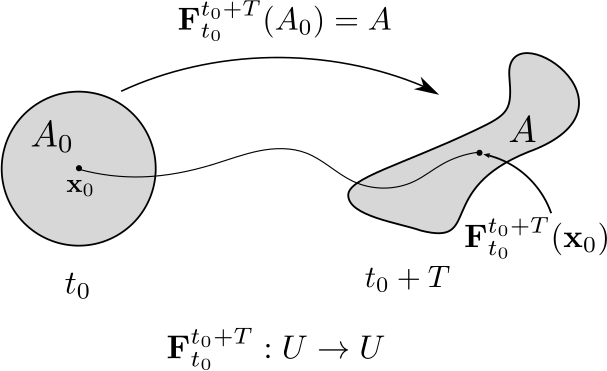
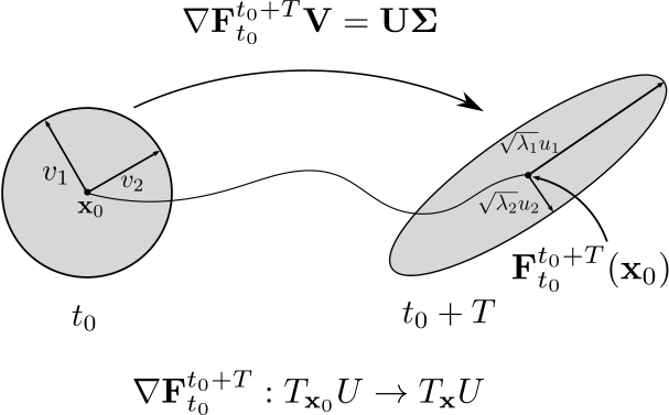
The figure on the left shows the action of the flow map on a small circle and the figure on the right shows the linear approximation. Let \(\nabla\mathbf{F}_{t_0}^{t_0 + T} = \mathbf{U\Sigma V^*}\) be the SVD of the linearized flow map. The singular values (diag (\(\mathbf{U}\))) are equal to the square root of the eigenvalues (\(\sqrt{\lambda_i}\)) of \(\mathbf{C}^{t_0+T}_{t_0}\) and the right singular vectors (\(v_i\)) are equal to the eigenvectors (\(\xi_i\)) of \(\mathbf{C}^{t_0+T}_{t_0}\).
Note
The flow map acts on elements of the domain and maps them to the domain. Its action on a set can be defined in the following manner: \(\mathbf{F}^{t_0 + T}_{t_0}(A_0) := \{\mathbf{F}^{t_0 + T}_{t_0}(\mathbf{x}_0) \in U | \mathbf{x}_0 \in A_0\}\). The derivative of the flow map, \(\nabla\mathbf{F}^{t_0+T}_{t_0}\), acts on elements of the tangent space (i.e. vectors) and maps them to elements of the tangent space downstream at \(\mathbf{x}=\mathbf{F}_{t_0}^{t_0 + T}(\mathbf{x}_0)\).
FTLE
The finite time Lyapunov exponent (FTLE), a finite time version of the classic Lyapunov exponent, is defined as,
FTLE was the first proposed method to find LCS [2], [3], [4] and remains a preferred method by many due to its relative simplicity to compute and its robustness to uncertainty in the underlying velocity data [5]. Regions of high FTLE are good indicators of repelling LCS in forward time and attracting LCS in backward time. By extracting ridges from the FTLE field, one can obtain the sought after hyperbolic structures.
Variational LCS
Haller then proposed the variational theory of hyperbolic LCS [6] in which he defines LCS as material curves (or surfaces in 3D) that are maximally repelling or attracting, normal to the curve, over the finite time window of interest and relative to nearby material curves. Here we give their definition in 2D. Given we have a dynamical system as in eq (1) with flowmap (2) and resulting eigenvalues and eigenvectors of \(\mathbf{C}^{t_0+T}_{t_0}(\mathbf{x}_0)\) as in (4), let \(\gamma^*(t) \in U\) be a compact material curve which evolves over the interval \([t_0,t_0+T]\). Then, \(\gamma^*(t)\) is a repelling LCS (if \(T>0\)) or attracting LCS (if \(T<0\)) if and only if the following conditions hold for all \(\mathbf{x}_0 \in \gamma^*(t_0)\):
\(\lambda_1 (\mathbf{x}_0) \neq \lambda_2 (\mathbf{x}_0) >1;\)
\(\left< \mathbf{\xi}_2 (\mathbf{x}_0), \nabla^2 \lambda_2(\mathbf{x}_0) \mathbf{\xi}_2 (\mathbf{x}_0) \right> \leq 0;\)
\(\mathbf{\xi}_1 (\mathbf{x}_0) || \gamma^*(t_0);\)
\(\overline{\lambda}_2 (\gamma)\), the average of \(\lambda_2\) over a curve \(\gamma\), is maximal on \(\gamma^*(t_0)\) among all nearby curves \(\gamma\) satisfying \(\gamma || \mathbf{\xi}_1 (\mathbf{x}_0).\)
Farzmand and Haller [7] detail how to implement this theory numerically and the NumbaCS implementation follows this paper quite closely, with deviations on how initial conditions are choosen and some additional options for the user when it comes to comparing candidate LCS. In short, solution curves are computed in the minimum eigenvector field \(\xi_1\) (satisfying C) until conditions A,B are not satisfied for some continuous predefined length. Then, nearby solution curves obtained in this manner are compared to satisfy condition D.
Note
The numerical implementation of the variational method for hyperbolic LCS yields accurate, smooth curves and is the direct implementation of their definition, but this comes at the expense of a somewhat significant increase in computational cost and additional complexity for the user as, typically, parameters in the implementation need to be in a somewhat narrow window to produce satisfactory LCS. There is no way of determining these parameters a priori and therefore this challenge is passed to the user in a trial and error fashion. For this reason, it is generally suggested to use one of the FTLE ridge methods described below.
FTLE ridges
As mentioned previously, FTLE ridges often coincide with hyperbolic LCS and therefore, extracting FTLE ridges themselves can serve as an alternative to the variational method for hyperbolic LCS. It should be noted, that there are cases when FTLE ridges can result in false positives due to regions of high shear [8], [6] but these ridges can be filtered out by checking additional criteria. In addition, it is not a gaurentee that every hyperbolic LCS will be along a FTLE ridge and therefore the ridge methods could potentially miss some hyperbolic LCS. In practice, very often FTLE ridges are indeed hyperbolic LCS and the FTLE ridge method picks up most of the dominant structures.
The simplest approach to identify FTLE ridges is to simply threshold the FTLE field. By only looking at FTLE values above a certain threshold, regions of high attraction and repulsion can be obtained in a very straightforward manner. This does not result in a true codimension-1 ridge though as, in a 2D flow, a 2D region will generally be returned in which a true ridge resides. When one simply desires a visual of influential regions, this can be a good first step. Sometimes actual ridges are desired for a variety of reasons. With a ridge, quantities normal and tangent to the ridge can be computed and tracking of specific ridges is possible. Below we detail the methods used to extract these ridges.
FTLE ridge extraction methods follow the methods developed in the image processing community designed to extract ridges from images. In image processing, images are usually converted to gray scale and the gray values are essentially used as a discrete height function. Most methods suggest smoothing the data with a Gaussian, providing a scale-space representation. From there, first and second derivatives of this height function are computed, often with derivatives of the Gaussian, and these derivatives are used to extract differential geometric properties of the height field. These ridges are often referred to as height ridges (or sometimes, a second-derivative ridge). Given a height function \(f\) in 2 dimensions, height ridge points are defined as all \(\mathbf{x}_0 \in U\) such that,
\(\left<\nabla f,\eta_{max}\right> = 0\);
\(\left<\eta_{max},H_{f}\cdot \eta_{max} \right> < 0\)
where \(H_f\) denotes the Hessian of \(f\) at \(\mathbf{x}_0\), \(\eta_{max}\) is the eigenvector of the Hessian corresponding to the largest (in magnitude) eigenvalue (representing the direction normal to the ridge), and it is implied that all quantities are evaluated at \(\mathbf{x}_0\). The first condition guarantees that the point is at an extrema of \(f\) (in the \(\eta_{max}\) direction) and the second, that \(f\) is concave down (in the \(\eta_{max}\) direction). Shadden et al. [4] first defined second-derivative FTLE ridges with these ideas in mind, using the FTLE field \(\sigma\) as the height field. Later Haller [6] defined FTLE ridges in a similar fashion to height ridges but required \(\nabla \lambda_2\) be tangent to the ridge and replaced \(\eta_{max}\) with \(\xi_2\) in the second condition. Finally, Schindler et al [9] further refined the criteria by using \(\xi_2\) in the first condition (they referred to these as C-ridges), resulting in the most common defintion of FTLE ridges today,
\(\left<\nabla \sigma,\xi_{2}\right> = 0\);
\(\left<\xi_2,H_{\sigma}\cdot \xi_{2} \right> < 0\).
In a numerical context, finding points which satisfy condition 1 is challenging as a grid point will rarely be exactly on a ridge. If this condition is applied in a strict sense, often very few points will be identified as ridge points. If condition 1 is relaxed and instead the inner product is required to be below some tolerance in magnitude, points around (and sometimes on) a ridge are often found. Neither of these results are desirable. A contour generatoring algorithm is sometimes suggested (e.g. marching squares) to find zero curves of condition 1 but this comes with its own issues due to the orientation discontinuities of the eigenvector field. To get around these issues, NumbaCS follows an approach used by Steger [10] to extract ridges from images. This approach obtains ridge points with subpixel accuracy by Taylor expanding the height field at a grid point and using this expansion to find the zero of condition 1. In addition, NumbaCS follows the approach in Steger to link and order points which belong to the same ridge. NumbaCS also adds an additional step that connects ridges together if an endpoint of each is within some tolerance and the angle between the vector connecting the endpoints and the tangent at each endpoint is below another tolerance.
Note
An approach first proposed by Mathur et al. [11], and later revisted by Senatore and Ross [12] using a scale-space representation, called dynamical sharpening is another way to obtain accurate FTLE ridges that uses the fact the FTLE ridges are attractors of the gradient dynamical system given by,
While this approach does yield accurate ridges, we found that the approach implemented in NumbaCS achieves roughly the same level of accuracy at a significantly lower computational cost.
What conditions guarentee that a FTLE ridge is a hyperbolic LCS? Haller gave some conditions in [6] which would guarentee this and later, Karrasch [13] further simplified these conditions in the case of differentiable eigenvectors. He showed that, given \(\gamma\) is a FTLE ridge as defined above, if all \(\mathbf{x}_0 \in \gamma\) satisfy conditions A and C from the variational definition for hyperbolic LCS, then \(\gamma\) is a hyperbolic LCS. Given that \(\nabla \sigma\) approximates the tangent to the ridge and that \(\xi_1 \perp \xi_2\), condition C is satisfied in an approximate sense and then the method employed simply needs to only consider points at which \(\sigma > 0\) (equivalent to condition A).
Hyperbolic OECS
Hyperbolic OECS are defined in a similar manner to hyperbolic LCS but instead of being tied to some integration time and finite time window, they are instantaneous structures derived the velocity field at a specific instant in time. Much like hyperbolic LCS, they are domainant attracting and repelling material lines which have a great deal of influence over short time dynamics. Defined by Serra and Haller [14], they are derived from the Eulerian rate of strain tensor as introduced in (5) and serve as cores of short term hyperbolic behavior.
Variational OECS
Much like the variational theory for hyperbolic LCS, hyperbolic OECS are defined as solution curves in the eigenvector fields from \(\mathbf{S}(\mathbf{x}_0,t)\). The properties which define them are somewhat different though and described below. From [14], repelling OECS at time t are solution curves in the \(\mathbf{e}_1\) field such that the curve contains a local maxima of \(s_2\) but contains no other local maxima of \(s_2\). Attracting OECS at time t are solution curves in the \(\mathbf{e}_2\) field such that the curve contains a local minimum of \(s_1\) but contains no other local minima of \(s_1\). In the case of an incompressible 2D flow, \(s_1 = -s_2\) so their extrema will conincide. Therefore, the sought after structures are referred to as objective saddle points (generalizing the notion of classic saddle points in time-independent flows) and highlight cores of short term hyperbolic behavior. To compute them, identify all local maxima above a certain threshold, integrate in each eigenvector field until the magnitude of the instantaneous attraction (or repullsion) rate is not longer monotonically decreasing or the curve is longer than a preset length.
iLE
A few years later, Nolan et al. [15] showed that, in the limit as integration time goes to zero, the FTLE converges to the eigenvalues of the Eulerian rate of strain tensor with its sign determined by which direction the limit is taken it. They referred to this as the instantaneous Lyapunov exponent (iLE) and defined it as,
where the \(\pm\) denotes which direction the limit is taken in and the maximum and minimum eigenvalues of \(\mathbf{S}(\mathbf{x}_0,t)\) respectively. The iLE is meant to serve as a diagnostic (like the FTLE does in the finite time case) in the instantaneous case. Like the FTLE field, they defined iLE ridges in the same manner as they were defined in FTLE ridges with the FTLE field being replaced by the \(s_1\) or \(s_2\) field and the eigenvector of \(\mathbf{C}^{t_0+T}_{t_0}(\mathbf{x}_0)\) replaced by the corresponding eigenvector of \(\mathbf{S}(\mathbf{x}_0,t)\).
Elliptic LCS
Elliptic LCS are closed material curves which bound sets that remain coherent under the action of the flow. First defined by Haller and Beron-Vera [16] using a variational formulation, these are closed curves which uniformly stretch or contract by the same factor over some finite time window of interest. Computing these structures using the variational formulation comes with some challenges which we will not address here as we do not implement this method. Later, Serra and Haller [17] proposed a simpler and more efficient algorithm which uses the fact that these curves are closed null geodesics of the appropriate Lorentzian metrics. This approach improves on the numerical implementation of the variational approach by providing a simpler algorithm with greater efficiency. Shortly before this work, Haller et al. [18] defined the Lagrangian averaged vorticity deviation (LAVD) and provided yet another way to identify elliptic LCS. NumbaCS implements this approach as we found it to be the most efficient.
LAVD
The LAVD is an objective quantity used to find rotationally coherent Lagrangian vortices in a flow, whose boundaries coincide with elliptic LCS. Given a system (1) with corresponding flow map (2), the vorticity at any point \(\mathbf{x} \in U\) is given by \(\mathbf{\omega} = \nabla \times \mathbf{v}(\mathbf{x},t)\). Then, the instantaneous spatial mean of vorticity is given by,
where vol(\(\cdot\)) represents the volume (in 3D) or the area (in 2D) and \(dV\) represents either a volume or area element. Then, the LAVD is defined as,
To extract rotationally coherent vortices, local maxima of the LAVD field are identifed and the outermost convex closed level curves around each of these local maxima are extracted. The maxima are referred to as LAVD-based vortex centers and the outermost curves are referred to as LAVD-based elliptic LCS. Due to numerical inaccuracies and potential precision issues in the algorithm choosen to extract the level curves, often curves are not required to be strictly convex but have a very small convexity deficiency. NumbaCS implements this method and measures convexity deficiency by computing the relative difference in area between the candidate curve and its convex hull.
Elliptic OECS
Like the hyperbolic case, elliptic LCS have Eulerian counterparts defined in very similar ways but in terms of eigenvalues and eigenvectors of \(\mathbf{S}(\mathbf{x}_0,t)\) instead of \(\mathbf{C}^{t_0+T}_{t_0}(\mathbf{x}_0)\). In the Serra and Haller paper [17], they show, by replacing the right Cauchy Green deformation tensor with the Euerian rate of strain tensor, that the null geodesic approach works for the Eulerian case as well. In the Haller et al. paper [18] on LAVD, they also define a quantity for the Eulerian case, the instantaneous vorticity deviation (IVD). Like the LAVD, the outermost closed convex level curves can be used to extract elliptic OECS. NumbaCS implements this approach.
IVD
The IVD is defined as,
and it can be shown that the IVD is the limit of the LAVD as integration time goes to zero. The outermost closed convex level curves can be extracted in the same manner as is done for LAVD. The maxima are referred to as IVD-based vortex centers and the outermost curves are referred to as IVD-based elliptic OECS.
Flow map Composition
Typically, the most expensive portion of any finite-time coherent strucrure method is the step of particle integration required to solve (1) and obtain flow maps (2). If the coherent structure quantity to be computed is only desired at a single instant, there is not much one can do to cheapen this step aside from using more efficient solvers, relaxing error tolerances, or using a coarser grid. Often, the quantity of interest is desired in a time series though, rather than at just a single frame. When this is the case, Brunton and Rowley [19] noted that redundent computation is being performed in the particle integration step that could be circumvented by interpolating the flow map (see Figure 1 in the cited article for a clear picture of the redundancy). This is done by exploiting the semigroup property of the flow maps defined in equation (2),
where \(t_{N} = t_0 + T\) and the associative binary operation is the composition operation. Therefore, the flow map over some time window \([t_0,t_0+T]\) can be obtained by composing a collection of intermediate flow maps of shorter time windows. This is not very useful when only a single flow map is desired but if a time series of flow maps is needed, this can cut down the computational cost. Note that if a time series of FTLE was desired for times \({t_0,t_1,...,t_n}\), derived from flow maps over the following time windows \({[t_0,t_0+T], [t_1,t_1+T], ... , [t_n,t_n+T]}\), these could be computed as,
Clearly, for each full flow map \(\mathbf{F}_{t_k}^{t_k+T}\), all but the first intermediate flow map (\(\mathbf{F}_{t_k}^{t_{k+1}}\)) used to create this full flow map can be recycled and used to create the succesive flow map \(\mathbf{F}_{t_{k+1}}^{t_{k+1}+T}\). Given that the flow map is being computed on a grid \(\mathcal{G}\), it is necessary to interpolate each intermediate flow map (after the first) since, in general, \(\mathbf{F}_{t_k}^{t_{k+1}}(\mathcal{G}) \not\rightarrow \mathcal{G}\) and this will be the input to the next intermediate flow map. Therefore, Brunton and Rowley define the interpolation operator \(\mathcal{I}\) which acts on a discrete map \(\mathbf{F}_{\mathcal{G}_k} := \mathbf{F}_{t_k}^{t_{k+1}}(\mathcal{G})\) and returns the interpolated map, i.e.
and \(\mathcal{I}\mathbf{F}_k\) is the interpolated flow map \(\mathbf{F}_{t_k}^{t_{k+1}}\). Then, for any \(t_k \in \{t_0,t_1,...,t_n\}\)
They call this the unidirectional method and also define a bidirectional method. They show that the bidirectional method is not as accurate or as fast so we omit any further discussion here. In addition, they suggest an alternative method for storage of smaller composed intermediate flow maps called the multi-tier (as opposed to single-tier) method. NumbaCS implements the single-tier unidirectional method which is what was described above.
Warning
This method achieves the most computational savings when particles mapped under the action of the flow do not leave the domain on which the coherent structure method is being computed (i.e. if \(U_{D} \subset U\) is the coherent structure domain then \(\mathbf{F}\restriction U_{D}: U_{D} \rightarrow U_{D}\)). If this is not the case, the flow map would need to be computed on a larger domain and the computational savings would shrink (and eventually vanish as the domain grew). NumbaCS currently only implements the flow map composition method when the coherent structure domain is self contained.
References
George Haller. Transport Barriers and Coherent Structures in Flow Data: Advective, Diffusive, Stochastic and Active Methods. Cambridge University Press, 2023.
G. Haller and A.C. Poje. Finite time transport in aperiodic flows. Physica D: Nonlinear Phenomena, 119(3):352–380, 1998. doi:https://doi.org/10.1016/S0167-2789(98)00091-8.
G. Haller. Distinguished material surfaces and coherent structures in three-dimensional fluid flows. Physica D: Nonlinear Phenomena, 149(4):248–277, 2001. doi:https://doi.org/10.1016/S0167-2789(00)00199-8.
Shawn C. Shadden, Francois Lekien, and Jerrold E. Marsden. Definition and properties of lagrangian coherent structures from finite-time lyapunov exponents in two-dimensional aperiodic flows. Physica D: Nonlinear Phenomena, 212(3):271–304, 2005. doi:https://doi.org/10.1016/j.physd.2005.10.007.
A Badza, T. Mattner, and S. Balasuriya. How sensitive are lagrangian coherent structures to uncertainties in data? Physica D: Nonlinear Phenomena, 444:133580, 2023. doi:https://doi.org/10.1016/j.physd.2022.133580.
George Haller. A variational theory of hyperbolic lagrangian coherent structures. Physica D: Nonlinear Phenomena, 240(7):574–598, 2011. doi:https://doi.org/10.1016/j.physd.2010.11.010.
Mohammad Farazmand and George Haller. Computing Lagrangian coherent structures from their variational theory. Chaos: An Interdisciplinary Journal of Nonlinear Science, 22(1):013128, 03 2012. doi:10.1063/1.3690153.
G. Haller. Lagrangian coherent structures from approximate velocity data. Physics of Fluids, 14(6):1851–1861, 06 2002. doi:10.1063/1.1477449.
Benjamin Schindler, Ronald Peikert, Raphael Fuchs, and Holger Theisel. Ridge Concepts for the Visualization of Lagrangian Coherent Structures, pages 221–235. Springer Berlin Heidelberg, Berlin, Heidelberg, 2012. doi:10.1007/978-3-642-23175-9_15.
C. Steger. An unbiased detector of curvilinear structures. IEEE Transactions on Pattern Analysis and Machine Intelligence, 20(2):113–125, 1998. doi:10.1109/34.659930.
Manikandan Mathur, George Haller, Thomas Peacock, Jori E. Ruppert-Felsot, and Harry L. Swinney. Uncovering the lagrangian skeleton of turbulence. Phys. Rev. Lett., 98:144502, Apr 2007. doi:10.1103/PhysRevLett.98.144502.
Carmine Senatore and Shane D. Ross. Detection and characterization of transport barriers in complex flows via ridge extraction of the finite time lyapunov exponent field. International Journal for Numerical Methods in Engineering, 86(9):1163–1174, 2011. doi:https://doi.org/10.1002/nme.3101.
Daniel Karrasch. Comment on “a variational theory of hyperbolic lagrangian coherent structures, physica d 240 (2011) 574–598”. Physica D: Nonlinear Phenomena, 241(17):1470–1473, 2012. doi:https://doi.org/10.1016/j.physd.2012.05.008.
Mattia Serra and George Haller. Objective Eulerian coherent structures. Chaos: An Interdisciplinary Journal of Nonlinear Science, 26(5):053110, 05 2016. doi:10.1063/1.4951720.
Peter Nolan, Mattia Serra, and Shane Ross. Finite-time lyapunov exponents in the instantaneous limit and material transport. Nonlinear Dyn, 100:3825–3852, 2020. doi:10.1007/s11071-020-05713-4.
G. Haller and F. J. Beron-Vera. Coherent lagrangian vortices: the black holes of turbulence. Journal of Fluid Mechanics, 731:R4, 2013. doi:10.1017/jfm.2013.391.
Mattia Serra and George Haller. Efficient computation of null geodesics with applications to coherent vortex detection. Proceedings of the Royal Society A: Mathematical, Physical and Engineering Sciences, 473(2199):20160807, 2017. doi:10.1098/rspa.2016.0807.
G. Haller, A. Hadjighasem, M. Farazmand, and F. Huhn. Defining coherent vortices objectively from the vorticity. Journal of Fluid Mechanics, 795:136–173, 2016. doi:10.1017/jfm.2016.151.
Steven L. Brunton and Clarence W. Rowley. Fast computation of finite-time Lyapunov exponent fields for unsteady flows. Chaos: An Interdisciplinary Journal of Nonlinear Science, 20(1):017503, 01 2010. doi:10.1063/1.3270044.