User Guide

This section is meant to get the user aquinted with the functions in NumbaCS and make the workflow through the modules clear. For a simpler approach to get started with NumbaCS, a user may be better served by picking an example from the Examples Gallery to go through and refering to this section as questions arise. An overview of the theory behind the methods presented here is covered in the Theory and Implementation section.

Lagrangian

Performing Lagrangian diagnostics and feature extraction is done using a similar workflow. First, a flow needs to obtained in a form that works with the ODE solver used by NumbaCS (numbalsoda). Then, particle integration needs to be performed over the domain of interest. Following that, one of the methods can be applied to obtain the desired quantities.

Flows

To begin using NumbaCS for Lagrangian methods, the user needs to define a flow from which coherent structures will be obtained. This is all done through the numbacs.flows module. NumbaCS provides predefined flows that the user can retrieve and a simple interface for generating the interpolants needed for numerical velocity fields.

Predefined flows

To retrieve a predefined flow, the user can call the numbacs.flows.get_predefined_flow() function to get one of the predefined flows. Currently, the supported flows are “double_gyre”, “bickley_jet”, and “abc”. To retrieve the “double_gyre” flow,

# import the function
from math import copysign
import numpy as np
from numbacs.flows import get_predefined_flow

# define integration time
T = -10.0
int_direction = copysign(1, T)

# get function pointer for 'double_gyre'
funcptr, params, domain = get_predefined_flow('double_gyre',
                                               int_direction = int_direction
                                               return_default_params = True,
                                               return_domain = True
                                               parameter_description = True)

# set up grid with nx points in x-direction and ny in y-direction
nx,ny = 401,201
x = np.linspace(domain[0][0], domain[0][1], nx)
y = np.linspace(domain[1][0], domain[1][1], ny)

Predefined flows have parameters in their definition that can be modified. A default set of parameters can be returned by setting the keyword argument return_default_params = True (it is True by default). In addition, by setting parameter_description = True (it is False by default), a string will be returned that details what each element of the params array coincides with in the definition of the ODE for each flow. For reference, the ODE (streamfunction for bickley jet) corresponding to each flow are listed below.

Double Gyre

(1)\[\begin{split}\dfrac{dx}{dt} &= -\pi A \sin(\pi f)\cos(\pi y) - \alpha x + \eta\\ \dfrac{dy}{dt} &= \pi A \cos(\pi f)\sin(\pi y) \dfrac{df}{dx} - \alpha y + \eta\\ f(x,t) &= \epsilon \sin(\omega t + \psi)x^2 + (1 - 2\epsilon \sin(\omega t + \psi)x).\end{split}\]

Bickely Jet

(2)\[\begin{split}\psi(x,y,t) = U_0 L(-\tanh(y/L) + \text{sech}^2(y/L&)(A_1 \cos(k_1(x - c_1 t)\\ &+ A_2 \cos(k_2(x - c_2 t)\\ &+ A_3 \cos(k_3(x - c_3 t))\end{split}\]

Time-periodic ABC flow

(3)\[\begin{split}\dfrac{dx}{dt} &= (A + \alpha\sin(t))\sin(z) + C\cos(y)\\ \dfrac{dy}{dt} &= B\sin(x) + (A + \alpha\sin(t))\cos(z)\\ \dfrac{dz}{dt} &= C\sin(y) + B\cos(x)\end{split}\]

Numerical flows

To use a numerical velocity field, which could have been obtained either from numerical simulation or real world data, interpolants need to be created for the velocity components in each direction. First, the user needs to call numbacs.flows.get_interp_arrays_2D(), and then pass the objects returned from that function into numbacs.flows.get_flow_2D().

# import the function
from math import copysign
import numpy as np
from numbacs.flows import get_interp_arrays_2D, get_flow_2D

# load in qge velocity data and define domain
u = np.load('./data/qge/qge_u.npy')
v = np.load('./data/qge/qge_v.npy')
nt,nx,ny = u.shape
x = np.linspace(0,1,nx)
y = np.linspace(0,2,ny)
t = np.linspace(0,1,nt)

# define integration time
T = -0.05
params = np.array([copysign(1,T)])

# get arrays for interpolant
grid_vel, C_eval_u, C_eval_v = get_interp_arrays_2D(t, x, y, u, v)

# get function pointer for interpolant of qge velocity data
funcptr = get_flow_2D(grid_vel, C_eval_u, C_eval_v, extrap_mode='linear')

This will create a cubic interpolant of the velocity field. To create a linear interpolant, coefficient arrays do not need to computed so there is no need to call get_interp_arrays_2D(). The linear interpolant can be obtained by simply calling get_flow_linear_2D().

# import the function
from math import copysign
import numpy as np
from numbacs.flows import get_flow_linear_2D
from interpolation.splines import UCGrid

# load in qge velocity data and define domain
u = np.load('./data/qge/qge_u.npy')
v = np.load('./data/qge/qge_v.npy')
nt,nx,ny = u.shape
x = np.linspace(0,1,nx)
y = np.linspace(0,2,ny)
t = np.linspace(0,1,nt)

# define integration time
T = -0.05
params = np.array([copysign(1,T)])


# set grid and get function pointer for interpolant of qge velocity data
grid_vel = UCGrid((t[0],t[-1],nt),(x[0],x[-1],nx),(y[0],y[-1],ny))
funcptr = get_flow_linear_2D(grid_vel, u, v, extrap_mode='linear')

Note

Due to how NumbaCS implements the ODE solver from numbalsoda, if the user wishes to integrate in a different direction in time, they need to change the integration direction in the params array (in addition to changing the sign of T). In NumbaCS, the first element of the params array (for flows) always contains the integration direction so to do this, the user can simply reassign the element, params[0] = -params[0].

User defined flows

It is possible for the user to define a flow but this is somewhat more cumbersome than the other options due to the requirements of the form of the flow from numbalsoda and NumbaCS. That being said, it is not too difficult. Say one wants to code up the time-dependent version of the cellular flow,

\[\begin{split}\dfrac{dx}{dt} &= -A \cos(x + B \sin(\omega t))\sin(y) \\ \dfrac{dy}{dt} &= A \sin(x + B \sin(\omega t))\cos(y).\end{split}\]

To use this with NumbaCS (and interface with numbalsoda), this could be coded up as,

# necessary imports
from numba import cfunc
from numbalsoda import lsoda_sig
from math import cos, sin

# create C callback using 'cfunc' decorator and 'lsoda_sig' signature
@cfunc(lsoda_sig)
def cellular_rhs(t,y,dy,p)
        """
        Defines time-dependent cellular flow to work with NumbaCS

        p[0] = int_direction, p[1] = A, p[2] = B, p[3] = omega
        """
        tt = p[0]*t
        dy[0] = p[0]*(-p[1]*cos(y[0] + p[2]*sin(p[3]*tt))*sin(y[1]))
        dy[1] = p[0]*(p[1]*sin(y[0] + p[2]*sin(p[3]*tt))*cos(y[1]))

# get function pointer to pass into integration functions
funcptr = cellular_rhs.address

Then funcptr can be used to pass into functions from the numbacs.integration module as will be demonstrated below.

Note

It is important that the rhs function is in this form to work with NumbaCS (i.e., the integration direction is the first value for p, both the time variable and the velocity in each direction are multiplied by it). The reason for this is that the numbalsoda ODE solvers intially did not allow for integration backwards in time so this method was used to get around that. Later, this was fixed through the solve_ivp function which calls the DOP853 method, though this is a tiny bit slower than calling the method directly. Due to the large number of calls to the ODE solver required by NumbaCS, we adopt this minorly inconvinient implementation in exchange for lower computation time.

Integration

Once a flow has been obtained, the next step is to integrate particles through that flow. The main function used for this is numbacs.integration.flowmap_grid_2D(). This function will integrate a grid of particles given by the cartesian product of x and y and return an array which contains the final positions of that grid of particles which were initialized at t0 and integrated for a duration of T. An array must be passed in which stores the parameters for the given flow. For a flow obtained through numbacs.flows.get_predefined_flow(), the params array returned by that function can be used as the array needed by the flow map function. If the flow was obtained through numbacs.flows.get_flow_2D(), the parameter array should be an array which contains 1.0 (for integration forwards in time) or -1.0 (for integration backwards in time). Additional arguments are method which control the integration method used (options are 'dop853' (default) and 'lsoda'), rtol (default is 1e-6) and atol (default is 1e-8) for relative and absolute tolerances respectively. A variety of other functions which integrate a collection of points or a grid of points are also available, some of which will be mentioned in later sections. For the rest, the reader is referred to the numbacs.integration module for more details. An example of using numbacs.integration.flowmap_grid_2D() is shown below.

# necessary imports
from math import copysign
import numpy as np
from numbacs.flows import get_interp_arrays_2D, get_flow_2D
from numbacs.integration import flowmap_grid_2D
from numabcs.diagnostics import ftle_grid_2D
import matplot.pyplot as plt

# load in qge velocity data and define domain
u = np.load('./data/qge/qge_u.npy')
v = np.load('./data/qge/qge_v.npy')
nt,nx,ny = u.shape
x = np.linspace(0,1,nx)
y = np.linspace(0,2,ny)
t = np.linspace(0,1,nt)

dx = dx[1] - dx[0]
dy = dy[1] - dy[0]
dt = t[1] - t[0]

# define integration time
T = 0.1
params = np.array([copysign(1,T)])

# get arrays for interpolant
grid_vel, C_eval_u, C_eval_v = get_interp_arrays_2D(t, x, y, u, v)

# get function pointer for interpolant of qge velocity data
funcptr = get_flow_2D(grid_vel, C_eval_u, C_eval_v, extrap_mode='linear')

# set initial time at which to perform particle integration, integrate grid
t0 = 0.0
flowmap = flowmap_grid_2D(funcptr, t0, T, x, y, params)

Flow map Composition

NumbaCS implements another approach to particle integration detailed in Flow map Composition which achieves a substantial speed-up in exchange for a small loss of accuracy. Refer to the linked section for information about when this approach can be used and see Time series for examples of computational savings for some specific flows. To use this approach, the user first needs to call numbacs.integration.flowmap_composition_initial() which implements the initial particle integration and interpolation step. Following this, call numbacs.integration.flowmap_composition_step() to take care of the next intermediate particle integration and interpolation. The argument h controls the time spacing between intermediate flow maps. It is important that T/h is a natural number. An example which computes a time series of flow maps is shown below.

import numpy as np
from interpolation.splines import UCGrid
from numbacs.integration import (flowmap_grid_2D, flowmap_composition_initial,
                                 flowmap_composition_step)
from numbacs.flows import get_interp_arrays_2D, get_flow_2D
import matplotlib.pyplot as plt
import time
from math import copysign
import numba
from numba import njit, prange

# %%
# Get flow data
# --------------
# Load velocity data, set up domain, set the integration span and direction, create
# interpolant of velocity data and retrieve necessary arrays.

# load in qge velocity data
u = np.load('../../../data/qge/qge_u.npy')
v = np.load('../../../data/qge/qge_v.npy')

# set up domain
nt,nx,ny = u.shape
x = np.linspace(0,1,nx)
y = np.linspace(0,2,ny)
t = np.linspace(0,3,nt)
dx = x[1]-x[0]
dy = y[1]-y[0]

# set integration span and integration direction
t0 = 0.0
T = 0.1
params = np.array([copysign(1,T)])  # important this is an array of type float

# get interpolant arrays of velocity field
grid_vel, C_eval_u, C_eval_v = get_interp_arrays_2D(t, x, y, u, v)

# get flow to be integrated
funcptr = get_flow_2D(grid_vel, C_eval_u, C_eval_v, extrap_mode='linear')

# %%
# Set flowmap composition parameters
# ----------------------------------
h = 0.005
grid = UCGrid((x[0],x[-1],nx),(y[0],y[-1],ny))
n = 50
tspan = np.arange(t0, t0 + n*h, h)
# %%
# Flowmap composition
# -------------------
# Perform flowmap composition over tspan.

full_flowmaps = np.zeros((n,nx,ny,2),np.float64)
flowmap0, flowmaps, nT = flowmap_composition_initial(funcptr,t0,T,h,x,y,grid,params)
full_flowmaps[0,:,:,:] = flowmap0

for k in range(1,n):
    t0 = tspan[k] + T - h
    flowmap_k, flowmaps = flowmap_composition_step(flowmaps,funcptr,t0,h,nT,x,y,grid,params)
    full_flowmaps[k,:,:,:] = flowmap_k

This can be used with any diagnostic or extraction method (described below) which can result in very fast computation times. See Time series for examples.

Fintie-time Diagnostics/Extraction

These examples use a numerical velocity field to obtain the function pointer (funcptr) but the same procedure can be performed if the function pointer was obtained from a predefined or user defined flow.

FTLE

Computing FTLE and FTLE ridges with NumbaCS is simple and efficient. Both methods use the numbacs.integration.flowmap_grid_2D() in the integration step but use seperate functions from numbacs.diagnostics to obtain the desired quantities.

FTLE fields

The main function needed to compute FTLE fields is numbacs.diagnostics.ftle_grid_2D() which takes as arguments a flow map, the integration time, and the x and y grid spacing.

# necessary imports
from math import copysign
import numpy as np
from numbacs.flows import get_interp_arrays_2D, get_flow_2D
from numbacs.integration import flowmap_grid_2D
from numabcs.diagnostics import ftle_grid_2D
import matplot.pyplot as plt

# load in qge velocity data and define domain
u = np.load('./data/qge/qge_u.npy')
v = np.load('./data/qge/qge_v.npy')
nt,nx,ny = u.shape
x = np.linspace(0,1,nx)
y = np.linspace(0,2,ny)
t = np.linspace(0,1,nt)

dx = dx[1] - dx[0]
dy = dy[1] - dy[0]
dt = t[1] - t[0]

# define integration time
T = 0.1
params = np.array([copysign(1,T)])

# get arrays for interpolant
grid_vel, C_eval_u, C_eval_v = get_interp_arrays_2D(t, x, y, u, v)

# get function pointer for interpolant of qge velocity data
funcptr = get_flow_2D(grid_vel, C_eval_u, C_eval_v, extrap_mode='linear')

# set initial time at which to perform particle integration, integrate grid
t0 = 0.0
flowmap = flowmap_grid_2D(funcptr, t0, T, x, y, params)

# compute ftle over grid
ftle = ftle_grid_2D(flowmap, T, dx, dy)

#plot results
fig,ax = plt.subplots()
ax.contourf(x,y,ftle.T,levels=100)
ax.set_aspect('equal')

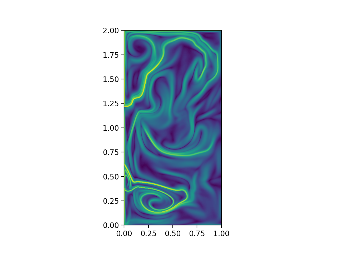
See FTLE for more examples.

FTLE ridges

To compute FTLE ridges, one needs to now use numbacs.diagnostics.C_eig_2D() to obtain the eigenvalues and eigenvectors of the Cauchy-Green strain tensor. The FTLE field is then computed using numbacs.diagnostics.ftle_from_eig().

Note

This is an alternative approach to compute the FTLE field to what was mentioned above, but if one is only interested in the field itself and not the ridges, the previously mentioned approach is slightly quicker as the eigenvectors are not computed and the FTLE formula is applied within the loop.

Three ridge detection methods are available that provide varying levels of detail, though they all implement the same base underlying method detailed in FTLE ridges.

First, the numbacs.extraction.ftle_ridge_pts() function can be used to identify all ridge points with subpixel accuracy. These points are not ordered and are not broken up into connected ridges. This is the fastest and can be used when one simply wants a visual of ridge points. Next, numbacs.extraction.ftle_ridges() provides the same ridge points with subpixel accuracy but this time breaks ridges up into connected structures, where a connected structure is a collection of points with continuous neighbors using an 8-grid neighborhood. These points are not ordered within each ridge. This can be useful when focus on a specific ridge is important and determining if a portion of the ridge is perhaps over some portion or feature of the domain. This is the next fastest. Finally, numbacs.extraction.ftle_ordered_ridges() extracts ridge points with subpixel accuracy, identifies connected ridges using a point linking algorithm, returns these points in an ordered fashion from one endpoint of the ridge to the other, and links ridges that have endpoints within some distance tolerance and are “in-line” (i.e. the angle between the tangent at each endpoint and the vector connecting the endpoints are below some tolerance). This is useful when order matters or when one wants to compute quantities normal or tangent to the ridge. This is the slowest but that is not to say it is slow, all of these methods are quite efficient after their first function call.

In all of these functions, the percentile and sdd_thresh arguments control which points are checked to be ridge points. Any points with a FTLE value below that percentile of the FTLE field will be ignored. The same goes for points with a second directional derivative (in the direction of the maximum eigenvector) value below sdd_thresh. For both numbacs.extraction.ftle_ridges() and numbacs.extraction.ftle_ordered_ridges(), the argument min_ridge_pts controls the minimum number of ridge points allowed in a ridge. Ridges with fewer points will be discarded. For numbacs.extraction.ftle_ordered_ridges(), additional arguments dist_tol and ep_tan_ang determine how close endpoints of ridges have to be to be considered for linking and the maximum allowable angle between a tangent to the ridge at and endpoint and the vector connecting the two endpoints respectively.

import numpy as np
from math import copysign, pi
from numbacs.flows import get_interp_arrays_2D, get_flow_2D
from numbacs.integration import flowmap_grid_2D
from numbacs.diagnostics import C_eig_2D, ftle_from_eig
from numbacs.extraction import ftle_ridge_pts, ftle_ridges, ftle_ridge_curves
from scipy.ndimage import gaussian_filter
import matplotlib.pyplot as plt

# load in qge velocity data
u = np.load('./data/qge/qge_u.npy')
v = np.load('./data/qge/qge_v.npy')
nt,nx,ny = u.shape
x = np.linspace(0,1,nx)
y = np.linspace(0,2,ny)
t = np.linspace(0,3,nt)

dx = x[1]-x[0]
dy = y[1]-y[0]

# set integration span and integration direction
t0 = 0.0
T = 0.1
params = np.array([copysign(1,T)])

# get ode to be used by 'flowmap_grid_2D'
grid_vel, C_eval_u, C_eval_v = get_interp_arrays_2D(t, x, y, u, v)
funcptr = get_flow_2D(grid_vel, C_eval_u, C_eval_v, extrap_mode='linear')

# computes final position of particle trajectories over grid
flowmap = flowmap_grid_2D(funcptr, t0, T, x, y, params)

# compute eigenvalues and eigenvectors of CG tensor over grid
eigvals,eigvecs = C_eig_2D(flowmap,dx,dy)

eigval_max = eigvals[:,:,1]
eigvec_max = eigvecs[:,:,:,1]

# copmute FTLE from max eigenvalue
ftle = ftle_from_eig(eigval_max,T)

# smooth ftle field
sigma = 1.2
ftle = gaussian_filter(ftle,sigma,mode='nearest')

percentile = 50
sdd_thresh = 10.0
# identify ridge points
ridge_pts = ftle_ridge_pts(ftle,eigvec_max,x,y,percentile=percentile,sdd_thresh=sdd_thresh)

# identify ridge points and break up by connected regions
ridges = ftle_ridges(ftle,eigvec_max,x,y,percentile=percentile,sdd_thresh=sdd_thresh)

# identify ridge points and link points in each ridge in an ordered manner
dist_tol = 5e-2
ep_tan_ang = pi/3
ridge_curves = ftle_ridge_curves(ftle,eigvec_max,x,y,dist_tol,
                                percentile=percentile,sdd_thresh=sdd_thresh,
                                ep_tan_ang=ep_tan_ang,min_ridge_pts=25)

# plot results
fig,axs = plt.subplots(nrows=1,ncols=3,sharey=True,dpi=300)
axs[0].contourf(x,y,ftle.T,levels=100)
axs[0].scatter(ridge_pts[:,0],ridge_pts[:,1],1.5,'r',marker='.',edgecolors=None,linewidths=0)
axs[0].set_aspect('equal')

axs[1].contourf(x,y,ftle.T,levels=100)
for r in ridges:
    axs[1].scatter(r[:,0],r[:,1],1.5,marker='.',edgecolors=None,linewidths=0)
axs[1].set_aspect('equal')

axs[2].contourf(x,y,ftle.T,levels=100)
k=0
for rc in ridge_curves:
    axs[2].plot(rc[:,0],rc[:,1],lw=0.5)

    k+=1
axs[2].set_aspect('equal')

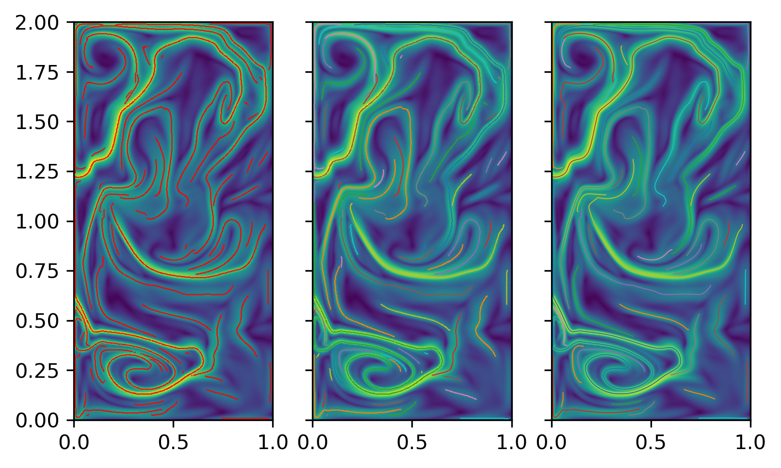
See FTLE for more examples.

Hyperbolic LCS

To extract hyperbolic LCS via the variational theory, particle integration needs to be performed on an auxillary grid in addition to the main grid. This is done by calling the numbacs.integration.flowmap_aux_grid_2D() function. Following this, numbacs.diagnostics.C_eig_aux_2D() needs to be called to return eigenvalues and eigenvectors of the Caughy Green strain tensor. By default, eigenvalues are computed from the main grid and eigenvectors are computed from the auxillary grid and this is controlled by the eig_main argument. Finally, hyperbolic LCS are computed using the numbacs.extraction.hyperbolic_lcs() function. This function has many parameters to be tuned and we will not detail them all here (refer to numbacs.extraction.hyperbolic_lcs() in the API reference for more details) though we will go over some of them. The argument dist_tol determines if candidate LCS curves will be compared and if so, how close they need to be at intersections with a coarse grid (controlled by nlines) to be compared. If dist_tol <= 0, then no comparison will be performed and all candiate LCS will be returned. Two other options for filtering are provided which are controlled by the arguments ep_dist_tol and arclen_flag. If ep_dist_tol > 0, curves which have an endpoint within this distance will be compared. Finally, arclen_flag determines how curves are compared. Traditionally, curves are compared by using the average normal attraction or repulsion rate. If arclen_flag == True, instead the total attraction or repulsion rate along a curve will be used to compare nearby curves. These last two methods for filtering are not standard but can sometimes provide a more satisfactory LCS picture (these are used in the double gyre example in the Hyperbolic LCS).

Note

There are certain flows which this method struggles with more than others. For example, it is challenging to get the parameters within an optimal window to filter candidate LCS satisfactorily for the QGE flow. Some curves stack up which could be lessened by increasing dist_tol or nlines, providing more filtering, though this would filter out desirable LCS as well. In addition, candidate curves occasionally appear “incorrect” for certain flows. It is not clear whether these issues are due to the NumbaCS implementation or the method struggling on specific applications. It is for these reasons, coupled with the additional computational cost compared to FTLE ridge methods, we generally suggest to use one of the FTLE ridge methods as long as the user is aware of and accepts the potential false positives and negatives mentioned in FTLE ridges. To see some examples of this method producing satisfactory results, refer to the Hyperbolic LCS section from the examples gallery.

# necessary imports
import numpy as np
from math import copysign
from numbacs.flows import get_interp_arrays_2D, get_flow_2D
from numbacs.integration import flowmap_aux_grid_2D
from numbacs.diagnostics import C_eig_aux_2D, ftle_from_eig
from numbacs.extraction import hyperbolic_lcs
import matplotlib.pyplot as plt

# load in qge velocity data
u = np.load('../../../data/qge/qge_u.npy')
v = np.load('../../../data/qge/qge_v.npy')

# set up domain
nt,nx,ny = u.shape
x = np.linspace(0,1,nx)
y = np.linspace(0,2,ny)
t = np.linspace(0,3,nt)
dx = x[1]-x[0]
dy = y[1]-y[0]

# set integration span and integration direction
t0 = 0.0
T = 0.1
params = np.array([copysign(1,T)])  # important this is an array of type float

# get interpolant arrays of velocity field
grid_vel, C_eval_u, C_eval_v = get_interp_arrays_2D(t, x, y, u, v)

# get flow to be integrated
funcptr = get_flow_2D(grid_vel, C_eval_u, C_eval_v, extrap_mode='linear')

# computes final position of particle trajectories over grid + auxillary grid
# with spacing h
h = 1e-4
flowmap = flowmap_aux_grid_2D(funcptr, t0, T, x, y, params,h=h)

# compute eigenvalues/vectors of Cauchy Green tensor
eigvals,eigvecs = C_eig_aux_2D(flowmap, dx, dy, h=h)
eigval_max = eigvals[:,:,1]
eigvec_max = eigvecs[:,:,:,1]

# copmute FTLE from max eigenvalue
ftle = ftle_from_eig(eigval_max,T)

# set parameters for hyperbolic lcs extraction,
# see function description for more details
step_size = 1e-3
steps = 3000
lf = 0.05
lmin = .25
r = 0.05
nmax = -1
dtol = 5e-2
nlines = 10
percentile = 60
ep_dist_tol = 0.0
lambda_avg_min = 0
arclen_flag = False

# extract hyperbolic lcs
lcs = hyperbolic_lcs(eigval_max, eigvecs, x, y, step_size, steps, lf, lmin, r, nmax,
                     dist_tol=dtol,
                     nlines=nlines,
                     ep_dist_tol=ep_dist_tol,
                     percentile=percentile,
                     lambda_avg_min=lambda_avg_min,
                     arclen_flag=arclen_flag)


# plot results
fig,ax = plt.subplots(dpi=200)
ax.contourf(x,y,ftle.T,levels=80)
for l in lcs:
    ax.plot(l[:,0],l[:,1],'r',lw=1)
ax.set_aspect('equal')

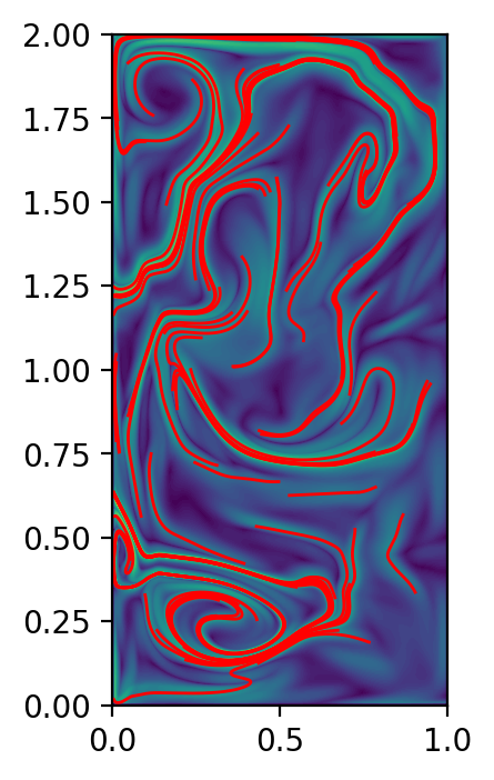
Elliptic LCS

The workflow to extract LAVD-based elliptic LCS is as follows. First, particle integration needs to be performed and the flow map must be returned at n times. This is done by the numbacs.integration.flowmap_n_grid_2D() function. This function will return the flow map at n equally spaced times in the time span \([t_0, t_0 + T]\) (inclusive) and will return the time span array corresponding to these times. In addition, the vorticity will need to be computed over the range of the flow maps and for the time span \([t_0, t_0 + T]\).

Note

While NumbaCS provides functions to compute vorticity, if dealing with a geophysical flow for which vorticity data is readily avaliable, it is recommended to use this data as it may be more accurate and will cut down on computational cost.

Vorticity can be computed from the velocity data itself (for a numerical flow) or from a function/interpolant of the velocity field (for either a predefined or numerical flow). The velocity interpolant can be created from either numbacs.flows.get_callable_2D() (cubic interpolant) or numbacs.flows.get_callable_linear_2D() (linear interpolant). To compute vorticity directly from velocity data, call numbacs.utils.curl_vel_tspan(). To compute vorticity from an interpolant, call numbacs.utils.curl_func_tspan(). After the vorticity is computed, an interpolant of it must be created which can be obtained by calling either numbacs.flows.get_callable_scalar() (cubic interpolant) or numbacs.flows.get_callable_scalar_linear() (linear interpolant).

Now LAVD can be computed using the numbacs.diagnostics.lavd_grid_2D() function. Following this, LAVD-based elliptic LCS (also known as rotationally coherent vortices) can be extracted using the numbacs.extraction.rotcohvrt() function. The argument r controls the radius in the numbacs.utils.max_in_radius() function. The convexity_deficiency argument controls the maximum allowed convexity deficiency for a curve to be considered an elliptic LCS. Finally, min_len controls the minimum allowed length for an elliptic LCS.

# necessary imports
import numpy as np
from math import copysign
import matplotlib.pyplot as plt
from numbacs.flows import (get_interp_arrays_2D, get_flow_2D, get_callable_2D,
                           get_interp_arrays_scalar, get_callable_scalar)
from numbacs.integration import flowmap_n_grid_2D
from numbacs.diagnostics import lavd_grid_2D
from numbacs.extraction import rotcohvrt
from numbacs.utils import curl_func_tspan

# load in qge velocity data
u = np.load('../../../data/qge/qge_u.npy')
v = np.load('../../../data/qge/qge_v.npy')

# set up domain
nt,nx,ny = u.shape
x = np.linspace(0,1,nx)
y = np.linspace(0,2,ny)
t = np.linspace(0,3,nt)
dx = x[1]-x[0]
dy = y[1]-y[0]

# set integration span and integration direction
t0 = 0.5
T = 0.3
params = np.array([copysign(1,T)])  # important this is an array of type float
n = 601

# get interpolant arrays of velocity field
grid_vel, C_eval_u, C_eval_v = get_interp_arrays_2D(t, x, y, u, v)

# get flow to be integrated
funcptr = get_flow_2D(grid_vel, C_eval_u, C_eval_v, extrap_mode='linear')

# get callable for flow
vel_spline = get_callable_2D(grid_vel, C_eval_u, C_eval_v, extrap_mode='linear')


# integrate grid of particles and return positions at n times between
# [t0,t0+T] (inclusive).
flowmap, tspan = flowmap_n_grid_2D(funcptr,t0,T,x,y,params,n=n)

# compute vorticity and create interpolant for it
vort = curl_func_tspan(vel_spline,tspan,x,y,h=1e-3)
grid_domain, C_vort = get_interp_arrays_scalar(tspan, x, y, vort)
vort_spline = get_callable_scalar(grid_domain, C_vort)

# need to pass raveled arrays into lavd_grid_2D
X,Y = np.meshgrid(x,y,indexing='ij')
xrav = X.ravel()
yrav = Y.ravel()

# compute lavd
lavd = lavd_grid_2D(flowmap, tspan, T, vort_spline, xrav, yrav)

# set parameters and compute lavd-based elliptic lcs
r = 0.2
convexity_deficiency = 1e-3
min_len = 0.1
elcs = rotcohvrt(lavd,x,y,r,convexity_deficiency=convexity_deficiency,min_len=min_len)

# plot the elliptic LCS over the LAVD field.
fig,ax = plt.subplots(dpi=200)
ax.contourf(x,y,lavd.T,levels=80)
ax.set_aspect('equal')
for rcv,c in elcs:
    ax.plot(rcv[:,0],rcv[:,1],lw=1.5)
    ax.scatter(c[0],c[1],1.5)

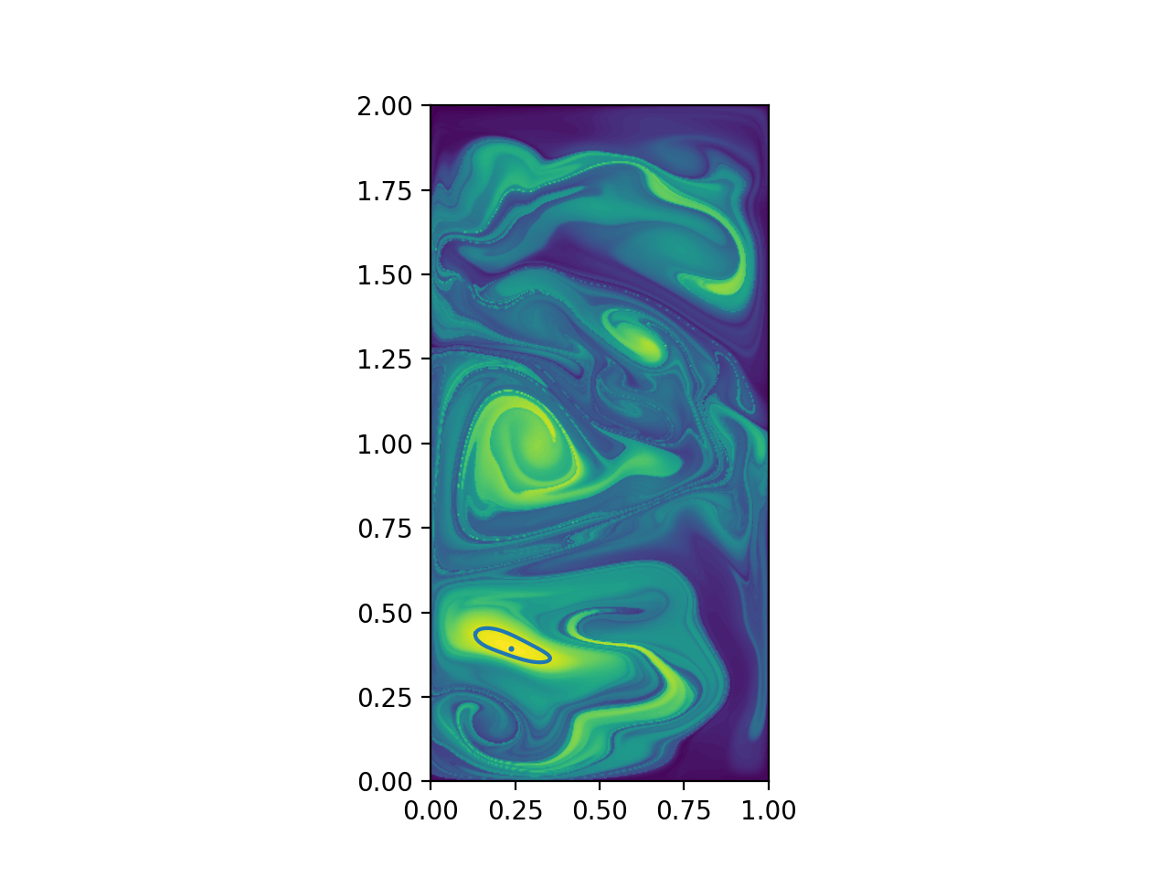
See Elliptic LCS for more examples.

Eulerian

Performing Eulerian diagnostics and feature extraction is done using a similar workflow. Since no particle integration is being performed, either the velocity data itself can be used (numerical flow with sufficient spatial resolution) or a callable needs to be obtained (predefined flow or numerical flow with insufficient spatial resolution). Following this, one of the methods can be applied to obtain the desired quantities.

Flows (callable)

To begin using NumbaCS for Eulerian methods, the user either needs to obtain a callable for the flow or use the velocity data itself. The same predefined flows from the Predefined flows section are available. The difference here is that the flows do not need to be able to interface with the numbalsoda package (numbalsoda requires that the right hand side of the ODE be a cfunc) but simply need to be able to be executed within Numba functions. The numbacs.flows module provides functions which can create/retrieve these for the user.

Predefined flows (callable)

To retrieve a callable for a predefined flow, the user can call the numbacs.flows.get_predefined_callable() function.

# necessary imports
from math import copysign
import numpy as np
from numbacs.flows import get_predefined_callable

# retrieve velocity func, domain, and parameter description
# for double gyre flow.
vel_func, domain, p_str = get_predefined_callable('double_gyre',
                                                  parameter_description=True)

# set up grid with nx points in x-direction and ny in y-direction
nx,ny = 401,201
x = np.linspace(domain[0][0],domain[0][1],nx)
y = np.linspace(domain[1][0],domain[1][1],ny)

Note

As mentioned in the Lagrangian section, predefined flows have paramters in their definition. Since no particle integration needs to be performed, int_direction is no longer the first element of the parameter array. By setting parameter_description = True, the description of a parameter array for a given flow can be seen.

Numerical flows (callable)

If the user has numerical velocity data and the domain over which its defined is not of sufficient spatial resolution, interpolants can be created for the velocity components in each direction and a callable can be returned. First, the user needs to call numbacs.flows.get_interp_arrays_2D(), and then pass the objects returned from that function into numbacs.flows.get_callable_2D().

# import the function
from math import copysign
import numpy as np
from numbacs.flows import get_interp_arrays_2D, get_callable_2D

# load in qge velocity data and define domain
u = np.load('./data/qge/qge_u.npy')
v = np.load('./data/qge/qge_v.npy')
nt,nx,ny = u.shape
x = np.linspace(0,1,nx)
y = np.linspace(0,2,ny)
t = np.linspace(0,1,nt)

# get arrays for interpolant
grid_vel, C_eval_u, C_eval_v = get_interp_arrays_2D(t, x, y, u, v)

# get callable for interpolant of qge velocity data
vel_func = get_callable_2D(grid_vel, C_eval_u, C_eval_v, spherical = 0, extrap_mode='linear')

This will create a cubic interpolant of the velocity field. To create a linear interpolant, coefficient arrays do not need to computed so this can be done by calling get_callable_linear_2D().

# import the function
from math import copysign
import numpy as np
from numbacs.flows import get_callable_linear_2D
from interpolation.splines import UCGrid

# load in qge velocity data and define domain
u = np.load('./data/qge/qge_u.npy')
v = np.load('./data/qge/qge_v.npy')
nt,nx,ny = u.shape
x = np.linspace(0,1,nx)
y = np.linspace(0,2,ny)
t = np.linspace(0,1,nt)

# set grid and get callable for interpolant of qge velocity data
grid_vel = UCGrid((t[0],t[-1],nt),(x[0],x[-1],nx),(y[0],y[-1],ny))
vel_func = get_callable_linear_2D(grid_vel, u, v, spherical = 0, extrap_mode='linear')

Note

For both predefined and numerical flows, the keyword argument return_type controls what the retrieved callable will return. To retrieve a callable which can be used by the Eulerian diagnostics functions in NumbaCS, return_type = 'array' needs to be set (it is this value be default). The callable retrieved with this argument will only take a single point as an input (point = [ti, xi, yi] where point is a np.array and ti, xi, yi are the t, x, and y values at which the velocity will be returned at). Sometimes, it may be useful to evaluate the velocity field at many points at once (perhaps to visualize the velocity field). This could be achieved with a loop with the callable mentioned above which only takes one point but it would not be efficient. For this purpose, setting return_type = 'tuple' will allow the user to pass many points (or a single point) at once in an efficient manner. Be aware that this callable type will not work with the Eulerian diagnostic functions from NumbaCS.

User defined flows (callable)

It is simpler for the user to define a flow used for Eulerian diagnostics as it no longer needs to interface with numbalsoda. If one wants to code up the time-dependent version of the cellular flow from User defined flows,

\[\begin{split}\dfrac{dx}{dt} &= -A \cos(x + B \sin(\omega t))\sin(y) \\ \dfrac{dy}{dt} &= A \sin(x + B \sin(\omega t))\cos(y).\end{split}\]

# necessary imports
from numba import njit
from math import cos, sin

# create jit-callable
@njit
def cellular(y)
        """
        Defines time-dependent cellular flow to work with NumbaCS
        for Eulerian diagnostics

        p[0] = A, p[1] = B, p[2] = omega
        """

        dx = -p[0]*cos(y[1] + p[1]*sin(p[2]*y[0]))*sin(y[2])
        dy = p[0]*sin(y[1] + p[1]*sin(p[2]*y[0]))*cos(y[2])

        return np.array([dx,dy],np.float64)

Now cellular can be used in place of vel_func in previous examples from this section. It is important that p is an array in memory which contains the values in the function description.

Instantaneous Diagnostics/Extraction

As mentioned, Eulerian diagnostics can be computed from a function representing the velocity field or from numerical data on a grid. NumbaCS has functions which can perform the diagnostics in either case. For the first diagnostic (iLE), we will demonstrate both cases but only show the numerical data case for the remaining methods.

iLE

For a velocity function, the numbacs.diagnostics.ile_2D_func() function needs to be called.

# necessary imports
import numpy as np
from numbacs.flows import get_interp_arrays_2D, get_callable_2D
from numbacs.diagnostics import ile_2D_func

# load in qge velocity data and define domain
u = np.load('./data/qge/qge_u.npy')
v = np.load('./data/qge/qge_v.npy')
nt,nx,ny = u.shape
x = np.linspace(0,1,nx)
y = np.linspace(0,2,ny)
t = np.linspace(0,1,nt)

# get arrays for interpolant
grid_vel, C_eval_u, C_eval_v = get_interp_arrays_2D(t, x, y, u, v)

# get callable for interpolant of qge velocity data
vel_func = get_callable_2D(grid_vel, C_eval_u, C_eval_v, spherical = 0, extrap_mode='linear')

# compute ile over grid at t = t0
t0 = t[15]
ile = ile_2D_func(vel_func,x,y,t0=t0)

Or iLE can be computed directly from the velocity data, which will be quicker but potentially less accurate (in this example, the grid which the data is defined on is sufficiently resolved). To do this, call the numbacs.diagnostics.ile_2D_data() function.

# necessary imports
import numpy as np
from numbacs.diagnostics import ile_2D_data

# load in qge velocity data and define domain
u = np.load('./data/qge/qge_u.npy')
v = np.load('./data/qge/qge_v.npy')
nt,nx,ny = u.shape
x = np.linspace(0,1,nx)
y = np.linspace(0,2,ny)
t = np.linspace(0,1,nt)
dx = x[1] - x[0]
dy = y[1] - y[0]

# compute ile over grid at t = t[k]
k = 15
ile = ile_2D_data(u[k,:,:],v[k,:,:],dx,dy)

Hyperbolic OECS

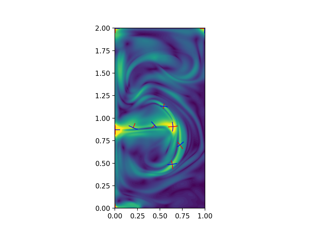
To extract hyperbolic OECS via the variational theory, eigenvalues and eigenvectors of the Eulerian rate of strain tensor need to be obtained. This can be done with either the numbacs.diagnostics.S_eig_2D_func() function for a velocity function or with the numbacs.diagnostics.S_eig_2D_data() for velocity data. Both of these functions have a handful of arguments which can be tuned to obtain different results. The argument r is the radius used in numbacs.utils.max_in_radius() function and will define the notion of “local” in the local maxima portion of the hyperbolic OECS definition. The argument maxlen defines the maximum length of a OECS curve, minval defines the minimum value allowed for the eigenvalue field – tensorline integration will stop when the eigenvalue field goes below this threshold. Finally n will determine how many local maxima will be used as initial conditions for generalized saddle points.

# necessary imports
import numpy as np
from numbacs.diagnostics import S_eig_2D_data
from numbacs.extraction import hyperbolic_oecs
import matplotlib.pyplot as plt

# load in qge velocity data
u = np.load('../../../data/qge/qge_u.npy')
v = np.load('../../../data/qge/qge_v.npy')

# set up domain
nt,nx,ny = u.shape
x = np.linspace(0,1,nx)
y = np.linspace(0,2,ny)
t = np.linspace(0,3,nt)
dx = x[1]-x[0]
dy = y[1]-y[0]

k0 = 15
# compute eigenvalues/vectors of Eulerian rate of strain tensor
eigvals,eigvecs = S_eig_2D_data(u[k0,:,:],v[k0,:,:],dx,dy)
s2 = eigvals[:,:,1]

# set parameters for hyperbolic_oecs function
r = 0.2
h = 1e-4
steps = 4000
maxlen = 0.05
minval = np.percentile(s2,50)
n = 10

# compute hyperbolic_oecs
oecs = hyperbolic_oecs(s2,eigvecs,x,y,r,h,steps,maxlen,minval,n=n)

# plot hyperbolic oecs overlaid on ile field
fig,ax = plt.subplots(dpi=200)
ax.contourf(x,y,s2.T,levels=np.linspace(0,np.percentile(s2,99.5),51),
            extend='both',zorder=0)

for k in range(len(oecs)):
    ax.plot(oecs[k][0][:,0],oecs[k][0][:,1],'r',lw=1)
    ax.plot(oecs[k][1][:,0],oecs[k][1][:,1],'b',lw=1)
ax.set_aspect('equal')

See Hyperbolic LCS for more examples.

Elliptic OECS

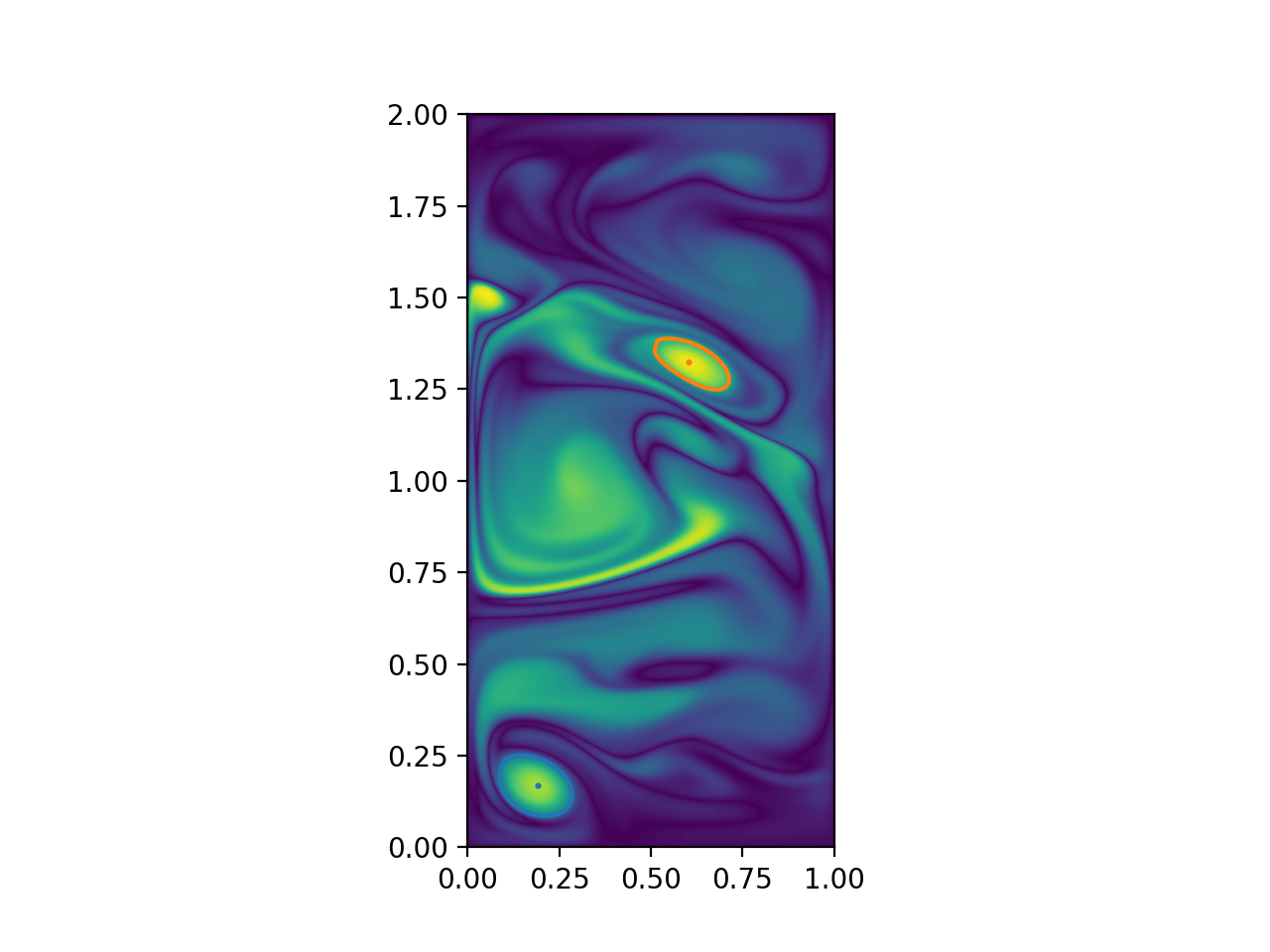
Extracting IVD-based elliptic OECS is similar to the process outlined for extracting Elliptic LCS but without the particle integration being performed. In this case, vorticity only needs to be computed at an instant and it is not necessary to interpolate the vorticity. Once the vorticity is obtained, simply compute the spatial mean. Then, call the numbacs.diagnostics.ivd_grid_2D() function to compute IVD. Following this, numbacs.extraction.rotcohvrt() can be called just like in the Lagrangian case as this function works for both LAVD and IVD, with arguments detailed in the Elliptic LCS section.

# necessary imports
import numpy as np
import matplotlib.pyplot as plt
from numbacs.diagnostics import ivd_grid_2D
from numbacs.extraction import rotcohvrt
from numbacs.utils import curl_vel

# load in qge velocity data
u = np.load('../../../data/qge/qge_u.npy')
v = np.load('../../../data/qge/qge_v.npy')

# set up domain
nt,nx,ny = u.shape
x = np.linspace(0,1,nx)
y = np.linspace(0,2,ny)
t = np.linspace(0,3,nt)
dx = x[1]-x[0]
dy = y[1]-y[0]

# set initial time
t0 = 0.5
k0 = np.argwhere(t==t0)[0][0]

# compute vorticity and spatial mean of vorticity
vort = curl_vel(u[k0,:,:],v[k0,:,:],dx,dy)
vort_avg = np.mean(vort)

# compute ivd
ivd = ivd_grid_2D(vort,vort_avg)

# set parameters and compute ivd-based elliptic oecs
r = 0.2
convexity_deficiency = 1e-3
min_len = 0.25
elcs = rotcohvrt(ivd,x,y,r,convexity_deficiency=convexity_deficiency,min_len=min_len)

# plot the elliptic OECS over the IVD field.
fig,ax = plt.subplots(dpi=200)
ax.contourf(x,y,ivd.T,levels=80)
ax.set_aspect('equal')
for rcv,c in elcs:
    ax.plot(rcv[:,0],rcv[:,1],lw=1.5)
    ax.scatter(c[0],c[1],1.5)

See Elliptic OECS for more examples.