Quasi-geostrophic Elliptic LCS

Compute the LAVD-based elliptic lcs for the QGE.

# Author: ajarvis
# Data: We thank Changhong Mou and Traian Iliescu for providing us with this dataset
#       and allowing it to be used here.

import numpy as np
from math import copysign
import matplotlib.pyplot as plt
from matplotlib.animation import FuncAnimation
from numbacs.flows import (
    get_interp_arrays_2D,
    get_flow_2D,
    get_callable_2D,
    get_interp_arrays_scalar,
    get_callable_scalar,
)
from numbacs.integration import flowmap_n_grid_2D, flowmap_n
from numbacs.diagnostics import lavd_grid_2D
from numbacs.extraction import rotcohvrt
from numbacs.utils import curl_func_tspan, gen_filled_circ, interp_curve, pts_in_poly_mask

Get flow data

Load velocity data, set up domain, set the integration span and direction, create interpolant of velocity data and retrieve necessary arrays.

# load in qge velocity data
u = np.load("../data/qge/qge_u.npy")
v = np.load("../data/qge/qge_v.npy")

# set up domain
nt, nx, ny = u.shape
x = np.linspace(0, 1, nx)
y = np.linspace(0, 2, ny)
t = np.linspace(0, 1, nt)
dx = x[1] - x[0]
dy = y[1] - y[0]

# set integration span and integration direction
t0 = 0.5
T = 0.3
params = np.array([copysign(1, T)])  # important this is an array of type float
n = 601

# get interpolant arrays of velocity field
grid_vel, C_eval_u, C_eval_v = get_interp_arrays_2D(t, x, y, u, v)

# get flow to be integrated
funcptr = get_flow_2D(grid_vel, C_eval_u, C_eval_v, extrap_mode="linear")

# get callable for flow
vel_spline = get_callable_2D(grid_vel, C_eval_u, C_eval_v, extrap_mode="linear")

Integrate

Integrate grid of particles and return positions at n times between [t0,t0+T] (inclusive).

flowmap, tspan = flowmap_n_grid_2D(funcptr, t0, T, x, y, params, n=n)

Vorticity

Copmute vorticity on the grid and over the times for which the flowmap was returned.

# compute vorticity and create interpolant for it
vort = curl_func_tspan(vel_spline, tspan, x, y, h=1e-3)
grid_domain, C_vort = get_interp_arrays_scalar(tspan, x, y, vort)
vort_spline = get_callable_scalar(grid_domain, C_vort)

LAVD

Compute LAVD from vorticity and particle positions.

# need to pass raveled arrays into lavd_grid_2D
X, Y = np.meshgrid(x, y, indexing="ij")
xrav = X.ravel()
yrav = Y.ravel()

# compute lavd
lavd = lavd_grid_2D(flowmap, tspan, T, vort_spline, xrav, yrav)

LAVD-based elliptic LCS

Compute elliptic LCS from LAVD.

# set parameters and compute lavd-based elliptic lcs
r = 0.2
convexity_deficiency = 1e-3
min_len = 0.1
elcs = rotcohvrt(lavd, x, y, r, convexity_deficiency=convexity_deficiency, min_len=min_len)

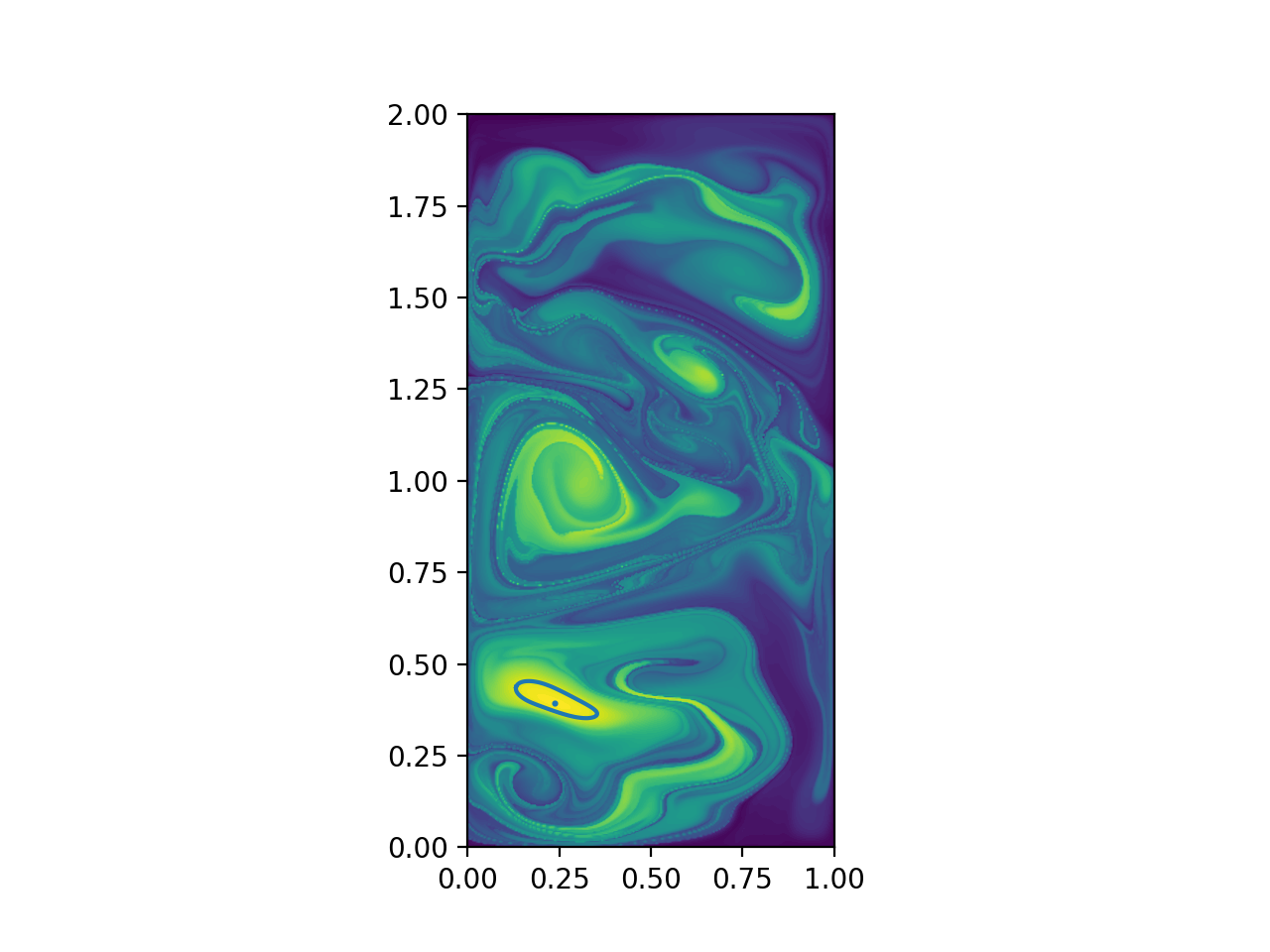
Plot

Plot the elliptic LCS over the LAVD field.

# sphinx_gallery_thumbnail_number = 1
fig, ax = plt.subplots(dpi=200)
ax.contourf(x, y, lavd.T, levels=80)
ax.set_aspect("equal")
for rcv, c in elcs:
    ax.plot(rcv[:, 0], rcv[:, 1], lw=1.5)
    ax.scatter(c[0], c[1], 1.5)
plt.show()

Advect elliptic LCS

Advect an elliptic LCS and nearby filled circle of points to demonstrate coherence.

# pick an elliptic lcs and create more refined curve by interpolating
c0 = elcs[0][1]
rcv0 = elcs[0][0]
rcvi = interp_curve(rcv0, 2500, per=1)

# create a filled circle which has a center a distance delta away from
# vortex center
delta = 1e-2
circ_delta = gen_filled_circ(0.1, 10000, c=c0 + delta, xlims=(0, 1), ylims=(0, 2))

# advect both the elliptic lcs and the nearby filled circle
frames = 301
adv_rcv, teval = flowmap_n(funcptr, t0, T, rcvi, params, n=frames)
adv_circ, _ = flowmap_n(funcptr, t0, T, circ_delta, params, n=frames)

Animate

Create animation of advected elliptic LCS and nearby filled circle.

# find which points from the filled circle are inside elliptic lcs
# for plotting purposes
mask = pts_in_poly_mask(rcv0, circ_delta)

# create plot
fig, ax = plt.subplots(dpi=100)
scatter0 = ax.scatter(adv_rcv[:, 0, 0], adv_rcv[:, 0, 1], 1)
scatter_in = ax.scatter(adv_circ[mask, 0, 0], adv_circ[mask, 0, 1], 0.5, "purple", zorder=0)
scatter_out = ax.scatter(adv_circ[~mask, 0, 0], adv_circ[~mask, 0, 1], 0.5, "orange", zorder=0)
ax.set_xlim([x[0], x[-1]])
ax.set_ylim([y[0], 1.25])  # only focus on part of domain where particles go
ax.set_aspect("equal")
ax.set_title(f"t = {round(teval[0], 2):.2f}")


# function for animation
def update(frame):
    # for each frame, update the data stored on each artist
    x0 = adv_rcv[:, frame, 0]
    y0 = adv_rcv[:, frame, 1]
    x_in = adv_circ[mask, frame, 0]
    y_in = adv_circ[mask, frame, 1]
    x_out = adv_circ[~mask, frame, 0]
    y_out = adv_circ[~mask, frame, 1]
    data0 = np.column_stack((x0, y0))
    data_in = np.column_stack((x_in, y_in))
    data_out = np.column_stack((x_out, y_out))

    # update each scatter plot
    scatter0.set_offsets(data0)
    scatter_in.set_offsets(data_in)
    scatter_out.set_offsets(data_out)

    # update title
    ax.set_title(f"t = {round(teval[frame], 2):.2f}")

    return (scatter0, scatter_in, scatter_out)


# create animation
ani = FuncAnimation(fig=fig, func=update, frames=frames, interval=30)
plt.show()

Once Loop Reflect