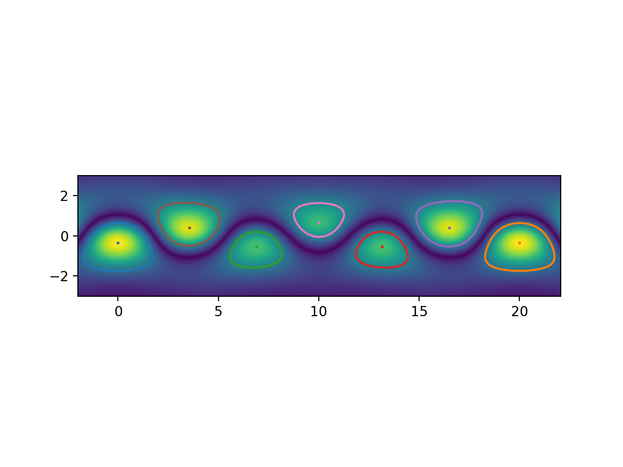
Bickley jet Elliptic OECS

Compute the IVD-based elliptic OECS for the Bickley jet.

# Author: ajarvis

import numpy as np
from math import pi
import matplotlib.pyplot as plt
from numbacs.flows import get_predefined_callable
from numbacs.diagnostics import ivd_grid_2D
from numbacs.extraction import rotcohvrt
from numbacs.utils import curl_func_tspan

Get flow callable

Get callable for velocity field, set up domain, and initial time

# retrieve callable to compute vorticity
vel_spline = get_predefined_callable("bickley_jet", return_domain=False)

# set up larger domain to capture all elliptic lcs
domain = ((-2.0, 6.371 * pi + 2.0), (-3.0, 3.0))
dx = 0.05
dy = 0.05
x = np.arange(domain[0][0], domain[0][1] + dx, dx)
y = np.arange(domain[1][0], domain[1][1] + dy, dy)
nx = len(x)
ny = len(y)

# set initial time
t0 = 0.0
t = np.array([t0])

Vorticity

Compute vorticity on the grid at t0.

# compute vorticity and spatial mean of vorticity
vort = curl_func_tspan(vel_spline, t, x, y).squeeze()
vort_avg = np.mean(vort)

IVD

Compute IVD from vorticity.

# compute lavd
ivd = ivd_grid_2D(vort, vort_avg)

IVD-based elliptic OECS

Compute elliptic OECS from IVD.

# set parameters and compute lavd-based elliptic oecs
r = 2.5
convexity_deficiency = 5e-6
min_len = 1.0
elcs = rotcohvrt(ivd, x, y, r, convexity_deficiency=convexity_deficiency, min_len=min_len)

Plot

Plot the elliptic OECS over the IVD field.

# sphinx_gallery_thumbnail_number = 1
fig, ax = plt.subplots(dpi=200)
ax.contourf(x, y, ivd.T, levels=80)
ax.set_aspect("equal")
for rcv, c in elcs:
    ax.plot(rcv[:, 0], rcv[:, 1], lw=1.5)
    ax.scatter(c[0], c[1], 1.5)
plt.show()