Quasi-geostrophic Elliptic OECS

Compute the IVD-based elliptic OECS for the QGE.

# Author: ajarvis
# Data: We thank Changhong Mou and Traian Iliescu for providing us with this dataset
#       and allowing it to be used here.

import numpy as np
import matplotlib.pyplot as plt
from numbacs.diagnostics import ivd_grid_2D
from numbacs.extraction import rotcohvrt
from numbacs.utils import curl_vel

Get flow data

Load velocity data, set up domain, and set initial time

# load in qge velocity data
u = np.load("../data/qge/qge_u.npy")
v = np.load("../data/qge/qge_v.npy")

# set up domain
nt, nx, ny = u.shape
x = np.linspace(0, 1, nx)
y = np.linspace(0, 2, ny)
t = np.linspace(0, 1, nt)
dx = x[1] - x[0]
dy = y[1] - y[0]

# set initial time
t0 = 0.5
k0 = np.argwhere(t == t0)[0][0]

Vorticity

Copmute vorticity on the grid and over the times for which the flowmap was returned.

# compute vorticity and create interpolant for it
vort = curl_vel(u[k0, :, :], v[k0, :, :], dx, dy)
vort_avg = np.mean(vort)

IVD

Compute IVD from vorticity.

# compute lavd
ivd = ivd_grid_2D(vort, vort_avg)

IVD-based elliptic OECS

Compute elliptic OECS from IVD.

# set parameters and compute lavd-based elliptic oecs
r = 0.2
convexity_deficiency = 1e-3
min_len = 0.25
elcs = rotcohvrt(ivd, x, y, r, convexity_deficiency=convexity_deficiency, min_len=min_len)

Plot

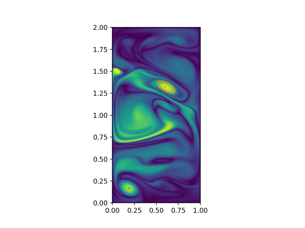
Plot the elliptic OECS over the IVD field.

# sphinx_gallery_thumbnail_number = 1
fig, ax = plt.subplots(dpi=200)
ax.contourf(x, y, ivd.T, levels=80)
ax.set_aspect("equal")
for rcv, c in elcs:
    ax.plot(rcv[:, 0], rcv[:, 1], lw=1.5)
    ax.scatter(c[0], c[1], 1.5)
plt.show()