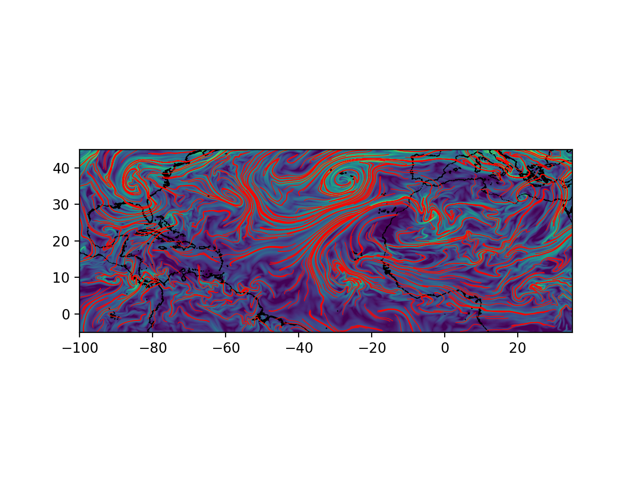
MERRA-2 Hyperbolic LCS

Compute hyperbolic LCS using the variational theory for atmospheric flow at time of Godzilla dust storm using MERRA-2 data which is vertically averaged over pressure surfaces ranging from 500hPa to 800hPa..

# Author: ajarvis
# Data: MERRA-2 - Global Modeling and Assimilation Office - NASA

import numpy as np
from math import copysign
from numbacs.flows import get_interp_arrays_2D, get_flow_2D
from numbacs.integration import flowmap_aux_grid_2D
from numbacs.diagnostics import C_eig_aux_2D, ftle_from_eig
from numbacs.extraction import hyperbolic_lcs
import matplotlib.pyplot as plt

Get flow data

Load in atmospheric velocity data, dates, and coordinates. Set domain for FTLE computation and integration span. Create interpolant and retrieve flow.

Note

Pandas is a simpler option for storing and manipulating dates but we use numpy here as Pandas is not a dependency.

# load in atmospheric data
dates = np.load("../data/merra_june2020/dates.npy")
dt = (dates[1] - dates[0]).astype("timedelta64[h]").astype(int)
t = np.arange(0, len(dates) * dt, dt, np.float64)
lon = np.load("../data/merra_june2020/lon.npy")
lat = np.load("../data/merra_june2020/lat.npy")

# NumbaCS uses 'ij' indexing, most geophysical data uses 'xy'
# indexing for the spatial coordintes. We need to switch axes and
# scale by 3.6 since velocity data is in m/s and we want km/hr.
u = np.moveaxis(np.load("../data/merra_june2020/u_500_800hPa.npy"), 1, 2) * 3.6
v = np.moveaxis(np.load("../data/merra_june2020/v_500_800hPa.npy"), 1, 2) * 3.6
nt, nx, ny = u.shape

# set domain on which ftle will be computed
dx = 0.1
dy = 0.1
lonf = np.arange(-100, 35 + dx, dx)
latf = np.arange(-5, 45 + dy, dy)


# set integration span and integration direction
day = 16
t0_date = np.datetime64(f"2020-06-{day:02d}")
t0 = t[np.nonzero(dates == t0_date)[0][0]]
T = -72.0
params = np.array([copysign(1, T)])

# get interpolant arrays of velocity field
grid_vel, C_eval_u, C_eval_v = get_interp_arrays_2D(t, lon, lat, u, v)

# set integration direction and retrieve flow
# set spherical = 1 since flow is on spherical domain and lon is from [-180,180)
params = np.array([copysign(1, T)])
funcptr = get_flow_2D(grid_vel, C_eval_u, C_eval_v, spherical=1)

Integrate

Integrate grid of particles and auxillary grid with spacing h, return final positions

# computes final position of particle trajectories over grid + auxillary grid
# with spacing h
h = 5e-3
flowmap = flowmap_aux_grid_2D(funcptr, t0, T, lonf, latf, params, h=h)

CG eigenvalues, eigenvectors, and FTLE

Compute eigenvalues/vectors of CG tensor from final particle positions and compute FTLE.

# compute eigenvalues/vectors of Cauchy Green tensor
eigvals, eigvecs = C_eig_aux_2D(flowmap, dx, dy, h=h)
eigval_max = eigvals[:, :, 1]
eigvec_max = eigvecs[:, :, :, 1]

# copmute FTLE from max eigenvalue
ftle = ftle_from_eig(eigval_max, T)

Hyperbolic LCS

Compute hyperbolic LCS using the variational theory.

# set parameters for hyperbolic lcs extraction,
# see function description for more details
step_size = 5e-3
steps = 10000
lf = 0.15
lmin = 5.0
r = 2.0
nmax = 2000
dtol = 0
nlines = 20
percentile = 0
ep_dist_tol = 0.0
lambda_avg_min = 0
arclen_flag = False

# extract hyperbolic lcs
lcs = hyperbolic_lcs(
    eigval_max,
    eigvecs,
    lonf,
    latf,
    step_size,
    steps,
    lf,
    lmin,
    r,
    nmax,
    dist_tol=dtol,
    nlines=nlines,
    ep_dist_tol=ep_dist_tol,
    percentile=percentile,
    lambda_avg_min=lambda_avg_min,
    arclen_flag=arclen_flag,
)

Plot

Plot the results.

coastlines = np.load("../data/merra_june2020/coastlines.npy")
fig, ax = plt.subplots(dpi=200)
ax.scatter(coastlines[:, 0], coastlines[:, 1], 1, "k", marker=".", edgecolors=None, linewidths=0)
ax.contourf(lonf, latf, ftle.T, levels=80, zorder=0)
for l in lcs:
    ax.plot(l[:, 0], l[:, 1], "r", lw=0.5)

ax.set_xlim([lonf[0], lonf[-1]])
ax.set_ylim([latf[0], latf[-1]])
ax.set_aspect("equal")
plt.show()