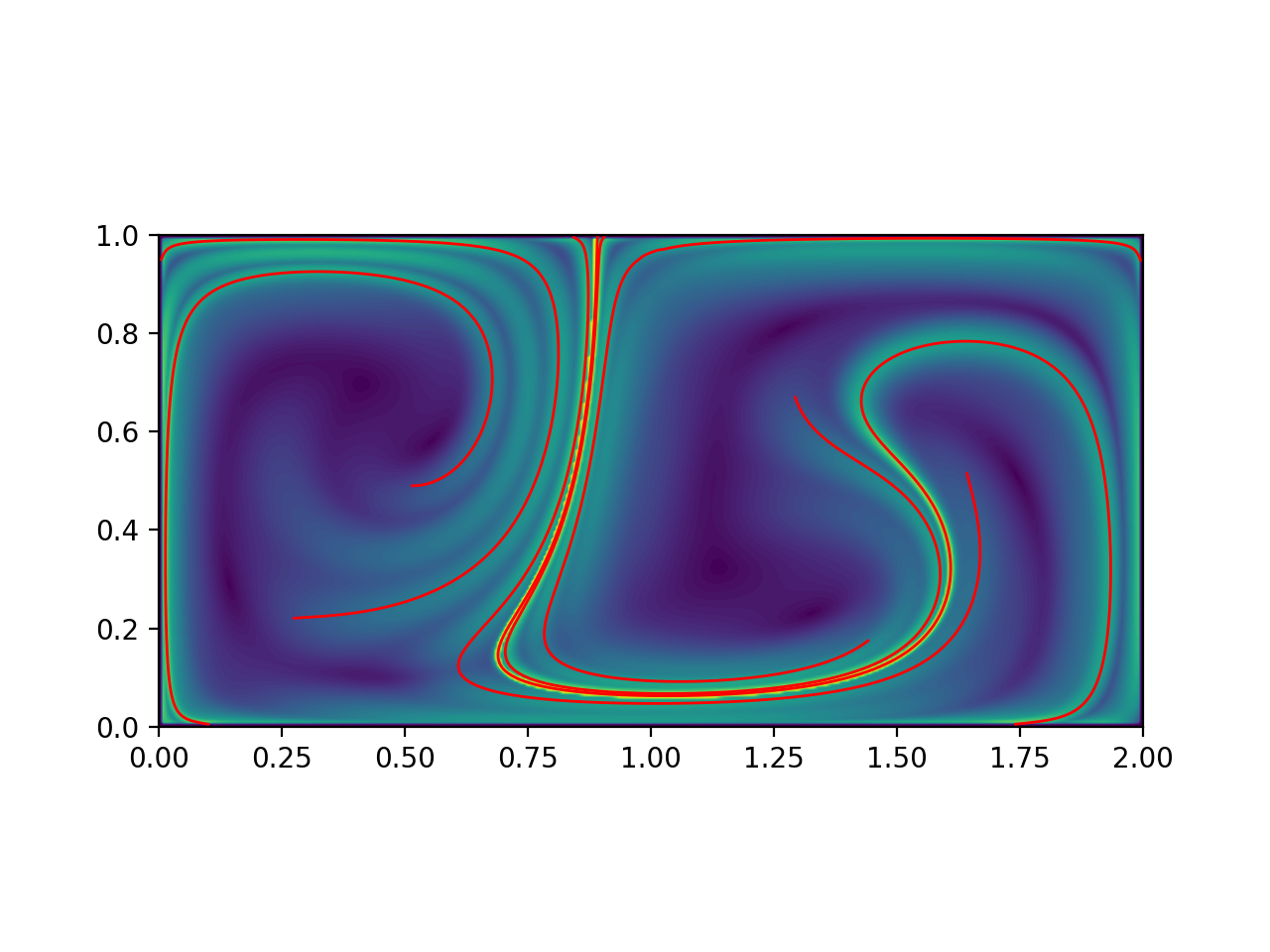
Double gyre Hyperbolic LCS

Compute hyperbolic LCS using the variational theory for the double gyre.

# Author: ajarvis

import numpy as np
from math import copysign
from numbacs.flows import get_predefined_flow
from numbacs.integration import flowmap_aux_grid_2D
from numbacs.diagnostics import C_eig_aux_2D, ftle_from_eig
from numbacs.extraction import hyperbolic_lcs
import matplotlib.pyplot as plt

Get flow

Set the integration span and direction, retrieve the flow, and set up domain.

# set initial time, integration time, and integration direction
t0 = 0.0
T = -10.0
int_direction = copysign(1, T)

# retrieve function pointer and parameters for double gyre flow.
funcptr, params, domain = get_predefined_flow("double_gyre", int_direction=int_direction)

# set up domain
nx, ny = 401, 201
x = np.linspace(domain[0][0], domain[0][1], nx)
y = np.linspace(domain[1][0], domain[1][1], ny)
dx = x[1] - x[0]
dy = y[1] - y[0]

Integrate

Integrate grid of particles and auxillary grid with spacing h, return final positions

# computes final position of particle trajectories over grid + auxillary grid
# with spacing h
h = 1e-5
flowmap = flowmap_aux_grid_2D(funcptr, t0, T, x, y, params, h=h)

CG eigenvalues, eigenvectors, and FTLE

Compute eigenvalues/vectors of CG tensor from final particle positions and compute FTLE.

# compute eigenvalues/vectors of Cauchy Green tensor
eigvals, eigvecs = C_eig_aux_2D(flowmap, dx, dy, h=h)
eigval_max = eigvals[:, :, 1]
eigvec_max = eigvecs[:, :, :, 1]

# copmute FTLE from max eigenvalue
ftle = ftle_from_eig(eigval_max, T)

Hyperbolic LCS

Compute hyperbolic LCS using the variational theory.

# set parameters for hyperbolic lcs extraction,
# see function description for more details
step_size = 1e-3
steps = 3000
lf = 0.1
lmin = 1.5
r = 0.1
nmax = -1
dtol = 1e-1
nlines = 10
percentile = 40
ep_dist_tol = 1e-2
lambda_avg_min = 600
arclen_flag = True

# extract hyperbolic lcs
lcs = hyperbolic_lcs(
    eigval_max,
    eigvecs,
    x,
    y,
    step_size,
    steps,
    lf,
    lmin,
    r,
    nmax,
    dist_tol=dtol,
    nlines=nlines,
    ep_dist_tol=ep_dist_tol,
    percentile=percentile,
    lambda_avg_min=lambda_avg_min,
    arclen_flag=arclen_flag,
)

Plot

Plot the results.

fig, ax = plt.subplots(dpi=200)
ax.contourf(x, y, ftle.T, levels=80)
for l in lcs:
    ax.plot(l[:, 0], l[:, 1], "r", lw=1)
ax.set_aspect("equal")
plt.show()