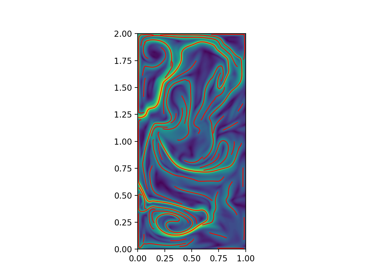
Quasi-geostrophic FTLE ridges

Compute the FTLE field and ridges for the QGE.

# Author: ajarvis
# Data: We thank Changhong Mou and Traian Iliescu for providing us with this dataset
#       and allowing it to be used here.

import numpy as np
from math import copysign
import matplotlib.pyplot as plt
from numbacs.flows import get_interp_arrays_2D, get_flow_2D
from numbacs.integration import flowmap_grid_2D
from numbacs.diagnostics import ftle_from_eig, C_eig_2D
from numbacs.extraction import ftle_ordered_ridges
from scipy.ndimage import gaussian_filter

Get flow data

Load velocity data, set up domain, set the integration span and direction, create interpolant of velocity data and retrieve necessary arrays.

# load in qge velocity data
u = np.load("../data/qge/qge_u.npy")
v = np.load("../data/qge/qge_v.npy")

# set up domain
nt, nx, ny = u.shape
x = np.linspace(0, 1, nx)
y = np.linspace(0, 2, ny)
t = np.linspace(0, 1, nt)
dx = x[1] - x[0]
dy = y[1] - y[0]

# set integration span and integration direction
t0 = 0.0
T = 0.1
params = np.array([copysign(1, T)])  # important this is an array of type float

# get interpolant arrays of velocity field
grid_vel, C_eval_u, C_eval_v = get_interp_arrays_2D(t, x, y, u, v)

# get flow to be integrated
funcptr = get_flow_2D(grid_vel, C_eval_u, C_eval_v, extrap_mode="linear")

Integrate

Integrate grid of particles and return final positions.

flowmap = flowmap_grid_2D(funcptr, t0, T, x, y, params)

CG eigenvalues, eigenvectors, and FTLE

Compute eigenvalues/vectors of CG tensor from final particle positions and compute FTLE.

# compute eigenvalues/vectors of Cauchy Green tensor
eigvals, eigvecs = C_eig_2D(flowmap, dx, dy)
eigval_max = eigvals[:, :, 1]
eigvec_max = eigvecs[:, :, :, 1]

# compute FTLE from max eigenvalue
ftle = ftle_from_eig(eigval_max, T)

# smooth ftle field, usually a good idea for numerical velocity field
sigma = 1.2
ftle_c = gaussian_filter(ftle, sigma, mode="nearest")

Ridge extraction

Compute ordered FTLE ridges.

# set parameters for ridge function
# function is fast after first call so experiment with these parameters
percentile = 50
sdd_thresh = 5e3

# identify ridge points, link points in each ridge in an ordered manner,
# connect close enough ridges
dist_tol = 5e-2
ridge_curves = ftle_ordered_ridges(
    ftle_c,
    eigvec_max,
    x,
    y,
    dist_tol,
    percentile=percentile,
    sdd_thresh=sdd_thresh,
    min_ridge_pts=25,
)

Plot

Plot the results.

fig, ax = plt.subplots(dpi=200)
ax.contourf(x, y, ftle_c.T, levels=80)
for rc in ridge_curves:
    ax.plot(rc[:, 0], rc[:, 1], "r", lw=1.0)
ax.set_aspect("equal")
plt.show()