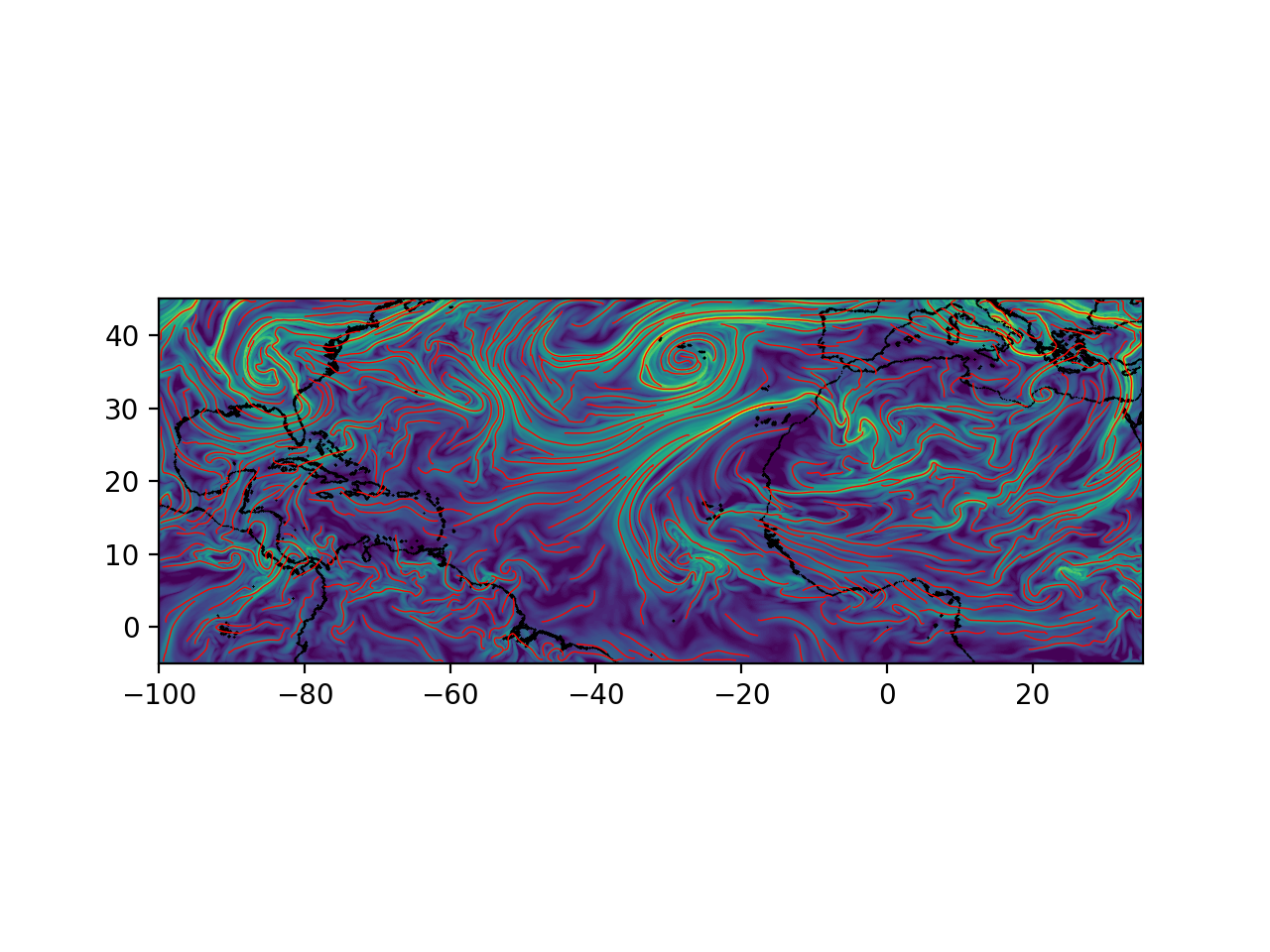
MERRA-2 FTLE ridges

Compute the FTLE field and ridges for atmospheric flow at time of Godzilla dust storm using MERRA-2 data which is vertically averaged over pressure surfaces ranging from 500hPa to 800hPa.

# Author: ajarvis
# Data: MERRA-2 - Global Modeling and Assimilation Office - NASA

import numpy as np
from math import copysign
import matplotlib.pyplot as plt
from numbacs.flows import get_interp_arrays_2D, get_flow_2D
from numbacs.integration import flowmap_grid_2D
from numbacs.diagnostics import C_eig_2D, ftle_from_eig
from numbacs.extraction import ftle_ordered_ridges
from scipy.ndimage import gaussian_filter

Get flow data

Load in atmospheric velocity data, dates, and coordinates. Set domain for FTLE computation and integration span. Create interpolant and retrieve flow.

Note

Pandas is a simpler option for storing and manipulating dates but we use numpy here as Pandas is not a dependency.

# load in atmospheric data
dates = np.load("../data/merra_june2020/dates.npy")
dt = (dates[1] - dates[0]).astype("timedelta64[h]").astype(int)
t = np.arange(0, len(dates) * dt, dt, np.float64)
lon = np.load("../data/merra_june2020/lon.npy")
lat = np.load("../data/merra_june2020/lat.npy")

# NumbaCS uses 'ij' indexing, most geophysical data uses 'xy'
# indexing for the spatial coordintes. We need to switch axes and
# scale by 3.6 since velocity data is in m/s and we want km/hr.
u = np.moveaxis(np.load("../data/merra_june2020/u_500_800hPa.npy"), 1, 2) * 3.6
v = np.moveaxis(np.load("../data/merra_june2020/v_500_800hPa.npy"), 1, 2) * 3.6
nt, nx, ny = u.shape

# set domain on which ftle will be computed
dx = 0.15
dy = 0.15
lonf = np.arange(-100, 35 + dx, dx)
latf = np.arange(-5, 45 + dy, dy)


# set integration span and integration direction
day = 16
t0_date = np.datetime64(f"2020-06-{day:02d}")
t0 = t[np.nonzero(dates == t0_date)[0][0]]
T = -72.0
params = np.array([copysign(1, T)])

# get interpolant arrays of velocity field
grid_vel, C_eval_u, C_eval_v = get_interp_arrays_2D(t, lon, lat, u, v)

# set integration direction and retrieve flow
# set spherical = 1 since flow is on spherical domain and lon is from [-180,180)
params = np.array([copysign(1, T)])
funcptr = get_flow_2D(grid_vel, C_eval_u, C_eval_v, spherical=1)

Integrate

Integrate grid of particles and return final positions.

flowmap = flowmap_grid_2D(funcptr, t0, T, lonf, latf, params)

CG eigenvalues, eigenvectors, and FTLE

Compute eigenvalues/vectors of CG tensor from final particle positions and compute FTLE.

# compute eigenvalues/vectors of Cauchy Green tensor
eigvals, eigvecs = C_eig_2D(flowmap, dx, dy)
eigval_max = eigvals[:, :, 1]
eigvec_max = eigvecs[:, :, :, 1]

# compute FTLE from max eigenvalue
ftle = ftle_from_eig(eigval_max, T)

# smooth ftle field, usually a good idea for numerical velocity field
sigma = 1.2
ftle_c = gaussian_filter(ftle, sigma, mode="nearest")

Ridge extraction

Compute ordered FTLE ridges.

# set parameters for ridge function
# function is fast after first call so experiment with these parameters
percentile = 30
sdd_thresh = 0.0

# identify ridge points, link points in each ridge in an ordered manner,
# connect close enough ridges
dist_tol = 5e-1
ridge_curves = ftle_ordered_ridges(
    ftle_c,
    eigvec_max,
    lonf,
    latf,
    dist_tol,
    percentile=percentile,
    sdd_thresh=sdd_thresh,
    min_ridge_pts=25,
)

Plot

Plot the results. Using the cartopy package for plotting geophysical data is advised but it is not a dependency so we simply use matplotlib.

coastlines = np.load("../data/merra_june2020/coastlines.npy")
fig, ax = plt.subplots(dpi=200)
ax.scatter(coastlines[:, 0], coastlines[:, 1], 1, "k", marker=".", edgecolors=None, linewidths=0)
ax.contourf(lonf, latf, ftle.T, levels=80, zorder=0)
for rc in ridge_curves:
    ax.plot(rc[:, 0], rc[:, 1], "r", lw=0.5)
ax.set_xlim([lonf[0], lonf[-1]])
ax.set_ylim([latf[0], latf[-1]])
ax.set_aspect("equal")
plt.show()