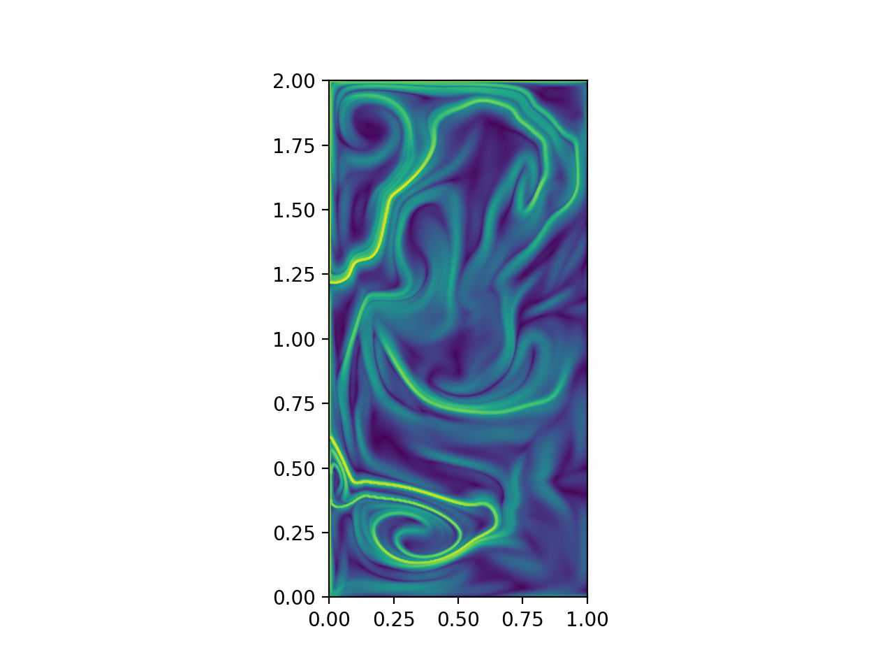
Quasi-geostrophic FTLE

Compute the FTLE field for the QGE.

# Author: ajarvis
# Data: We thank Changhong Mou and Traian Iliescu for providing us with this dataset
#       and allowing it to be used here.

import numpy as np
from math import copysign
import matplotlib.pyplot as plt
from numbacs.flows import get_interp_arrays_2D, get_flow_2D
from numbacs.integration import flowmap_grid_2D
from numbacs.diagnostics import ftle_grid_2D

Get flow data

Load velocity data, set up domain, set the integration span and direction, create interpolant of velocity data and retrieve necessary arrays.

# load in qge velocity data
u = np.load("../data/qge/qge_u.npy")
v = np.load("../data/qge/qge_v.npy")

# set up domain
nt, nx, ny = u.shape
x = np.linspace(0, 1, nx)
y = np.linspace(0, 2, ny)
t = np.linspace(0, 1, nt)
dx = x[1] - x[0]
dy = y[1] - y[0]

# set integration span and integration direction
t0 = 0.0
T = 0.1
params = np.array([copysign(1, T)])  # important this is an array of type float

# get interpolant arrays of velocity field
grid_vel, C_eval_u, C_eval_v = get_interp_arrays_2D(t, x, y, u, v)

# get flow to be integrated
funcptr = get_flow_2D(grid_vel, C_eval_u, C_eval_v, extrap_mode="linear")

Integrate

Integrate grid of particles and return final positions.

flowmap = flowmap_grid_2D(funcptr, t0, T, x, y, params)

FTLE

Compute FTLE field from final particle positions.

ftle = ftle_grid_2D(flowmap, T, dx, dy)

Plot

Plot the results.

fig, ax = plt.subplots(dpi=200)
ax.contourf(x, y, ftle.T, levels=100)
ax.set_aspect("equal")
plt.show()