MERRA-2 hyperbolic OECS

Compute the hyperbolic OECS saddles for atmospheric flow at time of Godzilla dust storm using MERRA-2 data which is vertically averaged over pressure surfaces ranging from 500hPa to 800hPa.

# Author: ajarvis
# Data: MERRA-2 - Global Modeling and Assimilation Office - NASA

import numpy as np
from numbacs.flows import get_interp_arrays_2D, get_callable_2D
from numbacs.diagnostics import S_eig_2D_func
from numbacs.extraction import hyperbolic_oecs
import matplotlib.pyplot as plt

Get flow data

Load in atmospheric velocity data, dates, and coordinates. Set domain for iLE computation, set time, and retrieve jit-callable function for velocity data.

Note

Pandas is a simpler option for storing and manipulating dates but we use numpy here as Pandas is not a dependency.

# load in atmospheric data
dates = np.load("../data/merra_june2020/dates.npy")
dt = (dates[1] - dates[0]).astype("timedelta64[h]").astype(int)
t = np.arange(0, len(dates) * dt, dt, np.float64)
lon = np.load("../data/merra_june2020/lon.npy")
lat = np.load("../data/merra_june2020/lat.npy")

# NumbaCS uses 'ij' indexing, most geophysical data uses 'xy'
# indexing for the spatial coordintes. We need to switch axes and
# scale by 3.6 since velocity data is in m/s and we want km/hr.
u = np.moveaxis(np.load("../data/merra_june2020/u_500_800hPa.npy"), 1, 2) * 3.6
v = np.moveaxis(np.load("../data/merra_june2020/v_500_800hPa.npy"), 1, 2) * 3.6
nt, nx, ny = u.shape

# set more refined domain on which iLE will be computed
dx = 0.15
dy = 0.15
lonf = np.arange(-35, 25 + dx, dx)
latf = np.arange(-5, 40 + dy, dy)


# get interpolant arrays of velocity field
grid_vel, C_eval_u, C_eval_v = get_interp_arrays_2D(t, lon, lat, u, v)

# get jit-callable interpolant of velocity data
vel_func = get_callable_2D(grid_vel, C_eval_u, C_eval_v, spherical=1)

# set time at which hyperbolic OECS will be computed
day = 20
t0_date = np.datetime64(f"2020-06-{day:02d}")
t0 = t[np.nonzero(dates == t0_date)[0][0]]

S eigenvalues, eigenvectors

Compute eigenvalues/vectors of S tensor from velocity field at time t = t0.

# compute eigenvalues/vectors of Eulerian rate of strain tensor
eigvals, eigvecs = S_eig_2D_func(vel_func, lonf, latf, h=1e-3, t0=t0)
s2 = eigvals[:, :, 1]

Hyperbolic OECS saddles

Compute generalized saddle points and hyperbolic oecs.

# set parameters for hyperbolic_oecs function
r = 5
h = 1e-3
steps = 4000
maxlen = 1.5
minval = np.percentile(s2, 50)
n = 10

# compute hyperbolic_oecs
oecs = hyperbolic_oecs(s2, eigvecs, lonf, latf, r, h, steps, maxlen, minval, n=n)

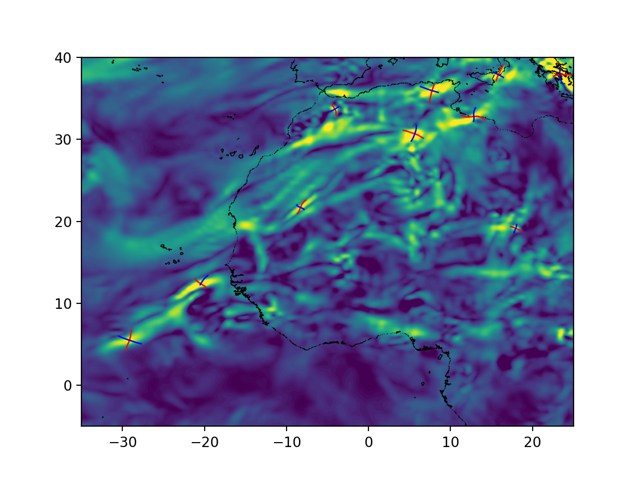
Plot all OECS

Plot the OECS overlaid on iLE.

Note

Cartopy is a useful package for geophysical plotting but it is not a dependency so we use matplotlib here.

coastlines = np.load("../data/merra_june2020/coastlines.npy")
fig, ax = plt.subplots(dpi=200)
ax.scatter(
    coastlines[:, 0], coastlines[:, 1], 1, "k", marker=".", edgecolors=None, linewidths=0, zorder=1
)
ax.contourf(
    lonf, latf, s2.T, levels=np.linspace(0, np.percentile(s2, 99.5), 51), extend="both", zorder=0
)

for k in range(len(oecs)):
    ax.plot(oecs[k][0][:, 0], oecs[k][0][:, 1], "r", lw=1)
    ax.plot(oecs[k][1][:, 0], oecs[k][1][:, 1], "b", lw=1)
ax.set_xlim([lonf[0], lonf[-1]])
ax.set_ylim([latf[0], latf[-1]])
ax.set_aspect("equal")
plt.show()

Advect OECS

Advect OECS and a circle centered at the generalized saddle point.

# import necessary functions
from numbacs.flows import get_flow_2D
from numbacs.utils import gen_filled_circ
from numbacs.integration import flowmap_n

# get funcptr, set parameters for integration, and integrate
funcptr = get_flow_2D(grid_vel, C_eval_u, C_eval_v, spherical=1)
nc = 1000
nT = 4
T = 24.0
t_eval = np.linspace(0, T, nT)
adv_circ = []
adv_rep = []
adv_att = []

# advect the top 3 (in strength) OECS
for k in range(len(oecs[:3])):
    circ1 = gen_filled_circ(r - 3.5, nc, c=oecs[k][2])
    adv_circ.append(flowmap_n(funcptr, t0, T, circ1, np.array([1.0]), n=nT)[0])
    adv_rep.append(flowmap_n(funcptr, t0, T, oecs[k][0], np.array([1.0]), n=nT)[0])
    adv_att.append(flowmap_n(funcptr, t0, T, oecs[k][1], np.array([1.0]), n=nT)[0])

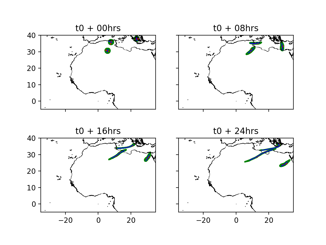
Plot advected OECS

Plot advected OECS at 0, 8, 16, and 24 hours after t0.

fig, axs = plt.subplots(nrows=2, ncols=2, sharex=True, sharey=True, dpi=200)
axs = axs.flat
nax = len(axs)
for i in range(nax):
    axs[i].scatter(
        coastlines[:, 0],
        coastlines[:, 1],
        1,
        "k",
        marker=".",
        edgecolors=None,
        linewidths=0,
        zorder=1,
    )
    kt = i
    axs[i].set_title(f"t0 + {round(t_eval[i]):02d}hrs")
    for k in range(len(adv_rep)):
        axs[i].scatter(
            adv_rep[k][:, kt, 0],
            adv_rep[k][:, kt, 1],
            1,
            "r",
            marker=".",
            edgecolors=None,
            linewidths=0,
        )
        axs[i].scatter(
            adv_att[k][:, kt, 0],
            adv_att[k][:, kt, 1],
            1,
            "b",
            marker=".",
            edgecolors=None,
            linewidths=0,
        )
        axs[i].scatter(adv_circ[k][:, kt, 0], adv_circ[k][:, kt, 1], 0.5, "g", zorder=0)
    axs[i].set_xlim([lonf[0], lonf[-1] + 10])
    axs[i].set_ylim([latf[0], latf[-1]])
    axs[i].set_aspect("equal")
plt.show()