MERRA iLE

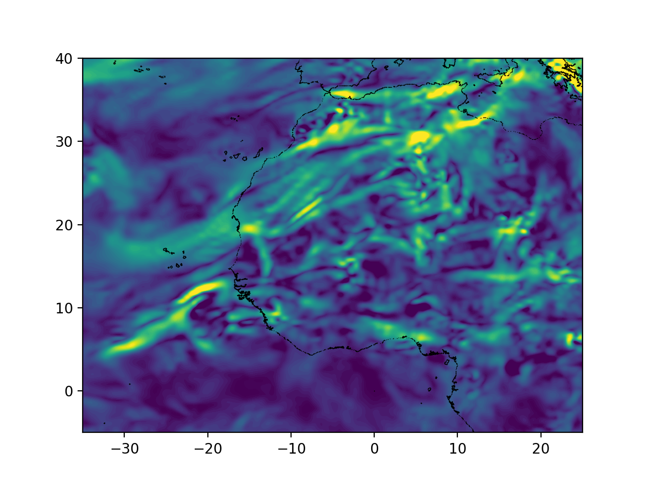
Compute the iLE field and for atmospheric flow at time of Godzilla dust storm using MERRA-2 data which is vertically averaged over pressure surfaces ranging from 500hPa to 800hPa.

# Author: ajarvis
# Data: MERRA-2 - Global Modeling and Assimilation Office - NASA

import numpy as np
import matplotlib.pyplot as plt
from numbacs.flows import get_interp_arrays_2D, get_callable_2D
from numbacs.diagnostics import ile_2D_func

Get flow data

Load in atmospheric velocity data, dates, and coordinates. Set domain for iLE computation, set time, and retrieve jit-callable function for velocity data.

Note

Pandas is a simpler option for storing and manipulating dates but we use numpy here as Pandas is not a dependency.

# load in atmospheric data
dates = np.load("../data/merra_june2020/dates.npy")
dt = (dates[1] - dates[0]).astype("timedelta64[h]").astype(int)
t = np.arange(0, len(dates) * dt, dt, np.float64)
lon = np.load("../data/merra_june2020/lon.npy")
lat = np.load("../data/merra_june2020/lat.npy")

# NumbaCS uses 'ij' indexing, most geophysical data uses 'xy'
# indexing for the spatial coordintes. We need to switch axes and
# scale by 3.6 since velocity data is in m/s and we want km/hr.
u = np.moveaxis(np.load("../data/merra_june2020/u_500_800hPa.npy"), 1, 2) * 3.6
v = np.moveaxis(np.load("../data/merra_june2020/v_500_800hPa.npy"), 1, 2) * 3.6
nt, nx, ny = u.shape

# set domain more refined domain on which iLE will be computed
dx = 0.15
dy = 0.15
lonf = np.arange(-35, 25 + dx, dx)
latf = np.arange(-5, 40 + dy, dy)

# get interpolant arrays of velocity field
grid_vel, C_eval_u, C_eval_v = get_interp_arrays_2D(t, lon, lat, u, v)

# get jit-callable interpolant of velocity data
vel_func = get_callable_2D(grid_vel, C_eval_u, C_eval_v, spherical=1)

# set time at which iLE will be computed
day = 20
t0_date = np.datetime64(f"2020-06-{day:02d}")
t0 = t[np.nonzero(dates == t0_date)[0][0]]

iLE

Compute iLE field from velocity data directly at time t0.

ile = ile_2D_func(vel_func, lonf, latf, t0=t0, h=1e-2)

Plot

Plot the results. Using the cartopy package for plotting geophysical data is advised but it is not a dependency so we simply use matplotlib.

coastlines = np.load("../data/merra_june2020/coastlines.npy")
fig, ax = plt.subplots(dpi=200)
ax.scatter(coastlines[:, 0], coastlines[:, 1], 1, "k", marker=".", edgecolors=None, linewidths=0)
ax.contourf(
    lonf, latf, ile.T, levels=np.linspace(0, np.percentile(ile, 99.5), 51), extend="both", zorder=0
)
ax.set_xlim([lonf[0], lonf[-1]])
ax.set_ylim([latf[0], latf[-1]])
ax.set_aspect("equal")
plt.show()