Quasi-geostraphic iLE

Compute the iLE field for the QGE.

# Author: ajarvis
# Data: We thank Changhong Mou and Traian Iliescu for providing us with this dataset
#       and allowing it to be used here.

import numpy as np
import matplotlib.pyplot as plt
from numbacs.diagnostics import ile_2D_data

Get flow data

Load velocity data and set up domain.

# load in qge velocity data
u = np.load("../data/qge/qge_u.npy")
v = np.load("../data/qge/qge_v.npy")

# set up domain
nt, nx, ny = u.shape
x = np.linspace(0, 1, nx)
y = np.linspace(0, 2, ny)
t = np.linspace(0, 1, nt)
dx = x[1] - x[0]
dy = y[1] - y[0]

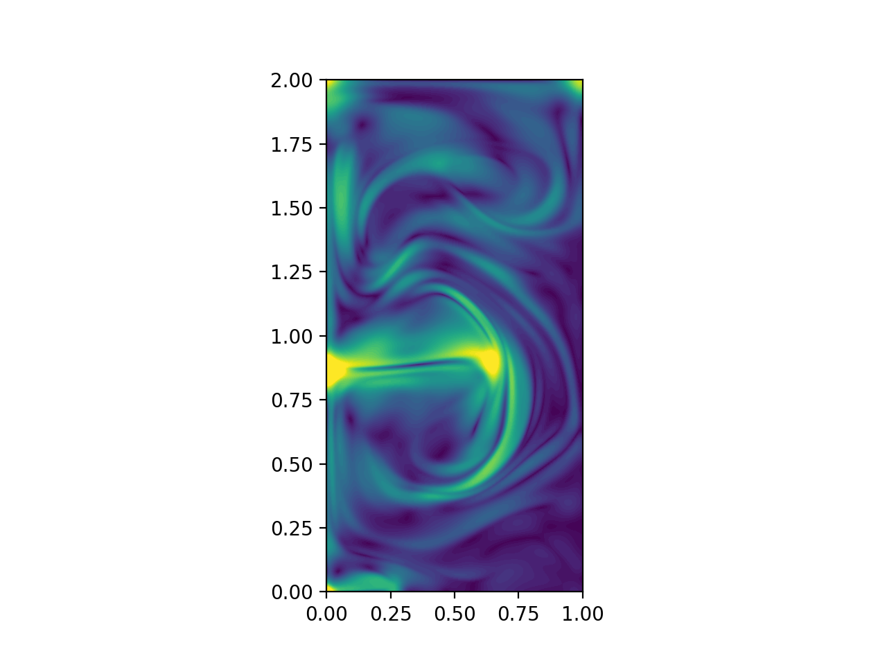
iLE

Compute iLE field from velocity data directly at time t[k].

k = 15
ile = ile_2D_data(u[k, :, :], v[k, :, :], dx, dy)

Plot

Plot the results.

fig, ax = plt.subplots(dpi=200)
ax.contourf(
    x, y, ile.T, levels=np.linspace(0, np.percentile(ile, 99.5), 51), extend="both", zorder=0
)
ax.set_aspect("equal")
plt.show()