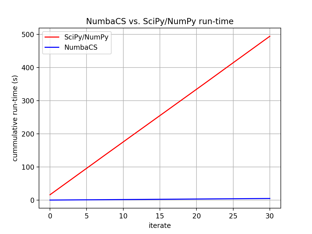
NumbaCS vs SciPy/NumPy – Double gyre

Compare run times for flow map and FTLE between NumbaCS and a pure SciPy/NumPy implementation for the double gyre.

# Author: ajarvis
# Hardware: Intel(R) Core(TM) i7-3770K CPU @ 3.50GHz, Cores = 4, Threads = 8

import numpy as np
from scipy.integrate import odeint
import matplotlib.pyplot as plt
from numbacs.integration import flowmap_grid_2D
from numbacs.flows import get_predefined_flow
from numbacs.diagnostics import ftle_grid_2D
import time
from math import pi, log
from multiprocessing import Pool
from functools import partial

Get flow for NumbaCS

Set the integration span and direction, retrieve the flow, and set up domain.

funcptr, params, domain = get_predefined_flow("double_gyre", int_direction=1.0)
nx = 201
ny = 101
x = np.linspace(domain[0][0], domain[0][1], nx)
y = np.linspace(domain[1][0], domain[1][1], ny)
dx = x[1] - x[0]
dy = y[1] - y[0]

t0 = 0.0
T = 16.0

Double Gyre for Scipy

Create function for SciPy ode solver.

A = 0.1
eps = 0.25
alpha = 0.0
omega = 0.2 * pi
psi = 0.0


def odeint_fun(yy, tt):
    """
    Function to represent double gyre flow to be used with odeint
    """

    a = eps * np.sin(omega * tt + psi)
    b = 1 - 2 * a
    f = a * yy[0] ** 2 + b * yy[0]
    df = 2 * a * yy[0] + b
    dx_ = -pi * A * np.sin(pi * f) * np.cos(pi * yy[1]) - alpha * yy[0]
    dy_ = pi * A * np.cos(pi * f) * np.sin(pi * yy[1]) * df - alpha * yy[1]

    return dx_, dy_

SciPy flow map and FTLE functions

Create functions to compute flow maps and FTLE using standard SciPy/Numpy methods. Uses scipy.integrate.odeint (implements LSODA method) for particle integration. The scipy.integrate.solve_ivp function is newer and allows the use of other solvers but odeint is faster even when solve_ivp uses LSODA as its method.

tspan = np.array([t0, t0 + T])


def scipy_odeint_flowmap_par(t0, y0):
    tspan = np.array([t0, t0 + T])
    sol = odeint(odeint_fun, y0, tspan, rtol=1e-6, atol=1e-8)
    flowmap = sol[-1, :]

    return flowmap


def numpy_ftle_par(fm, inds):
    i, j = inds
    absT = abs(T)
    dxdx = (fm[i + 1, j, 0] - fm[i - 1, j, 0]) / (2 * dx)
    dxdy = (fm[i, j + 1, 0] - fm[i, j - 1, 0]) / (2 * dy)
    dydx = (fm[i + 1, j, 1] - fm[i - 1, j, 1]) / (2 * dx)
    dydy = (fm[i, j + 1, 1] - fm[i, j - 1, 1]) / (2 * dy)

    off_diagonal = dxdx * dxdy + dydx * dydy
    C = np.array([[dxdx**2 + dydx**2, off_diagonal], [off_diagonal, dxdy**2 + dydy**2]])

    max_eig = np.linalg.eigvalsh(C)[-1]
    if max_eig > 1:
        ftle = 1 / (2 * absT) * log(max_eig)
    else:
        ftle = 0

    return ftle

Compute SciPy/Numpy flow map, FTLE

Compute flowmap, FTLE, and calculate run times for the SciPy/NumPy implementation. For this problem on this hardware, computing flow map and FTLE parallel in space (as opposed to parallel in time) was the faster implementation.

# set initial conditions
n = 31
t0span = np.linspace(0, 3, n)
[X, Y] = np.meshgrid(x, y, indexing="ij")
Y0 = np.column_stack((X.ravel(), Y.ravel()))
sftle = np.zeros((n, nx - 2, ny - 2), np.float64)

# set parallel pool to use maximum number of threads for this hardware,
# open pool
num_threads = 8
pl = Pool(num_threads)

# create inds to pass to ftle function
xinds = np.arange(1, nx - 1)
yinds = np.arange(1, ny - 1)
[I, J] = np.meshgrid(xinds, yinds, indexing="ij")
inds = np.column_stack((I.ravel(), J.ravel()))

# compute flowmap and ftle parallel in space
sfmtt = 0
sftt = 0
sfmtt_arr = np.zeros(n, np.float64)
sftt_arr = np.zeros(n, np.float64)

for k, t0 in enumerate(t0span):
    ks = time.perf_counter()
    func = partial(scipy_odeint_flowmap_par, t0)
    res = np.array(pl.map(func, Y0)).reshape(nx, ny, 2)
    kf = time.perf_counter()
    sfmtt += kf - ks
    sfmtt_arr[k] = sfmtt

    fks = time.perf_counter()
    func2 = partial(numpy_ftle_par, res)
    sftle[k, :, :] = np.array(pl.map(func2, inds)).reshape(nx - 2, ny - 2)
    fkf = time.perf_counter()
    sftt += fkf - fks
    sftt_arr[k] = sftt

pl.close()
pl.terminate()

print("SciPy/NumPy flowmap and FTLE took " + f"{sfmtt + sftt:.5f} seconds for {n} iterates")
print("Mean time for SciPy/NumPy flowmap and FTLE -- " + f"{(sfmtt + sftt) / n:.5f} seconds\n")
print(f"Scipy flowmap took {sfmtt:.5} seconds for {n:1d} iterates")
print(f"Mean time for Scipy flowmap -- {sfmtt / n:.5} seconds\n")
print(f"NumPy ftle took {sftt:.5} seconds for {n:1d} iterates")
print(f"Mean time for NumPy ftle -- {sftt / n:.5} seconds\n")

SciPy/NumPy flowmap and FTLE took 493.93187 seconds for 31 iterates
Mean time for SciPy/NumPy flowmap and FTLE -- 15.93329 seconds

Scipy flowmap took 488.92 seconds for 31 iterates
Mean time for Scipy flowmap -- 15.772 seconds

NumPy ftle took 5.0114 seconds for 31 iterates
Mean time for NumPy ftle -- 0.16166 seconds

Compute NumbaCS flow map, FTLE

Compute flowmap, FTLE, and calculate run times for the NumbaCS implementation. For this problem on this hardware, computing flow map and FTLE parallel in space (as opposed to parallel in time) was the faster implementation.

ftle = np.zeros((n, nx, ny), np.float64)

# first call and record warmup times
wfm = time.perf_counter()
flowmap_wu = flowmap_grid_2D(funcptr, t0, T, x, y, params)
wu_fm = time.perf_counter() - wfm
print(f"Flowmap with warm-up took {wu_fm:.5f} seconds")

wf = time.perf_counter()
ftle[0, :, :] = ftle_grid_2D(flowmap_wu, T, dx, dy)
wu_f = time.perf_counter() - wf
print(f"FTLE with warm-up took {wu_f:.5f} seconds\n")

# initialize runtime counters
fmtt = wu_fm
ftt = wu_f
fmtt_arr = np.zeros(n, np.float64)
ftt_arr = np.zeros(n, np.float64)
fmtt_arr[0] = fmtt
ftt_arr[0] = ftt

# loop over initial times, compute flowmap and ftle
for k, t0 in enumerate(t0span[1:]):
    ks = time.perf_counter()
    flowmap = flowmap_grid_2D(funcptr, t0, T, x, y, params)
    kf = time.perf_counter()
    kt = kf - ks
    fmtt += kt
    fmtt_arr[k + 1] = fmtt

    fks = time.perf_counter()
    ftle[k, :, :] = ftle_grid_2D(flowmap, T, dx, dy)
    fkf = time.perf_counter()
    ftt += fkf - fks
    ftt_arr[k + 1] = ftt

print("NumbaCS flowmap and FTLE took " + f"{fmtt + ftt:.5f} for {n:1d} iterates")
print(f"Mean time for flowmap and FTLE -- {(fmtt + fmtt) / n:.5f} seconds (w/ warmup)")
print(
    "Mean time for flowmap and FTLE -- "
    + f"{(fmtt - wu_fm + ftt - wu_f) / (n - 1):.5f} seconds (w/o warmup)\n"
)
print(f"NumbaCS flowmap_grid_2D took {fmtt:.5f} seconds for {n:1d} iterates")
print(f"Mean time for flowmap_grid_2D -- {fmtt / n:.5f} seconds (w/ warmup)")
print(
    "Mean time for flowmap_grid_2D -- " + f"{(fmtt - wu_fm) / (n - 1):.5f} seconds (w/o warmup)\n"
)
print(f"NumbaCS ftle_grid_2D took {ftt:.5f} seconds for {n:1d} iterates")
print(f"Mean time for ftle_grid_2D -- {ftt / n:.5f} seconds (w/ warmup)")
print("Mean time for ftle_grid_2D -- " + f"{(ftt - wu_f) / (n - 1):.5f} seconds (w/o warmup)")

Flowmap with warm-up took 0.15825 seconds
FTLE with warm-up took 0.00392 seconds

NumbaCS flowmap and FTLE took 4.94441 for 31 iterates
Mean time for flowmap and FTLE -- 0.31021 seconds (w/ warmup)
Mean time for flowmap and FTLE -- 0.15941 seconds (w/o warmup)

NumbaCS flowmap_grid_2D took 4.80828 seconds for 31 iterates
Mean time for flowmap_grid_2D -- 0.15511 seconds (w/ warmup)
Mean time for flowmap_grid_2D -- 0.15500 seconds (w/o warmup)

NumbaCS ftle_grid_2D took 0.13613 seconds for 31 iterates
Mean time for ftle_grid_2D -- 0.00439 seconds (w/ warmup)
Mean time for ftle_grid_2D -- 0.00441 seconds (w/o warmup)

Compare timings

Compare timings and quantify speed-up. The second and third columns quantify the speed-up gained using NumbaCS. The second column includes warm-up time, the speed-up would increase as n grows larger. The third column ignores the warm-up time and quantifies the speed-up as n goes to infinity and the warm-up time becomes negligible. This represents the theoretical speed-up.

stt = sfmtt + sftt
ntt = fmtt + ftt

stpi = (sfmtt + sftt) / n
ntpi = (ntt - wu_fm - wu_f) / (n - 1)

d1 = 5
d2 = 2
data = [
    [round(stt, d1), "--", "--"],
    [round(ntt, d1), round(stt / ntt, d2), round(stpi / ntpi, d2)],
]

times = [f"total time (n={n})", "speedup", "speedup (n->inf)"]
methods = ["SciPy/NumPy", "NumbaCS"]

format_row = "{:>25}" * (len(data[0]) + 1)

print(format_row.format("", *times))

for name, vals in zip(methods, data):
    print(format_row.format(name, *vals))

                   total time (n=31)                  speedup         speedup (n->inf)
SciPy/NumPy                493.93187                       --                       --
    NumbaCS                  4.94441                     99.9                    99.95

Plot run-time

fig, ax = plt.subplots(dpi=200)
ax.plot(sfmtt_arr + sftt_arr, "r")
ax.plot(fmtt_arr + ftt_arr, "b")
ax.set_xlabel("iterate")
ax.set_ylabel("cummulative run-time (s)")
ax.set_title("NumbaCS vs. SciPy/NumPy run-time")
ax.legend(["SciPy/NumPy", "NumbaCS"])
plt.grid()

Note

The standard SciPy/Numpy implementation could be made faster with additional packages. For example, by simply decorating odeint_fun with @njit, the SciPy integration can be sped up by roughly a factor of 6 (still roughly 20 times slower than numbalsoda/NumbaCS). This example is meant to demonstrate what a standard approach in Python might look like and give a rough estimate of the savings gained by using NumbaCS. The speed-up is largely achieved by the numbalsoda package which utilizes Numba.