Double gyre time series

Compare run times for different flowmap methods for the double gyre.

# Author: ajarvis
# Hardware: Intel(R) Core(TM) i7-3770K CPU @ 3.50GHz, Cores = 4, Threads = 8

import numpy as np
from interpolation.splines import UCGrid
from numbacs.integration import (
    flowmap_grid_2D,
    flowmap_composition_initial,
    flowmap_composition_step,
)
from numbacs.flows import get_predefined_flow
from numbacs.diagnostics import ftle_grid_2D
import matplotlib.pyplot as plt
import time
import numba
from numba import njit, prange

Get flow

Set the integration span and direction, retrieve the flow, and set up domain.

funcptr, params, domain = get_predefined_flow("double_gyre", int_direction=1.0)
nx = 201
ny = 101
x = np.linspace(domain[0][0], domain[0][1], nx)
y = np.linspace(domain[1][0], domain[1][1], ny)
dx = x[1] - x[0]
dy = y[1] - y[0]

t0 = 0.0
T = 16.0
h = 1.0
grid = UCGrid((x[0], x[-1], nx), (y[0], y[-1], ny))
n = 200
tspan = np.arange(t0, t0 + n * h, h)

Warm-up

Run flowmap_grid_2D and ftle_grid_2D so warm-up time is not included in comparison.

wu_t = time.perf_counter()
flowmap_wu = flowmap_grid_2D(funcptr, t0, T, x, y, params)
wu_t = time.perf_counter() - wu_t
print(f"Flowmap with warm-up took {wu_t:.5f} seconds")

wu_t = time.perf_counter()
ftle_wu = ftle_grid_2D(flowmap_wu, T, dx, dy)
wu_t = time.perf_counter() - wu_t
print(f"FTLE with warm-up took {wu_t:.5f} seconds")

Flowmap with warm-up took 0.14957 seconds
FTLE with warm-up took 0.00383 seconds

Flowmap composition

Perform flowmap composition over tspan and compute time series of FTLE.

ftlec = np.zeros((n, nx, ny), np.float64)
ctt = 0
c0s = time.perf_counter()
flowmap0, flowmaps, nT = flowmap_composition_initial(funcptr, t0, T, h, x, y, grid, params)
c0f = time.perf_counter()
c0 = c0f - c0s
ctt += c0

ftt = 0
f0s = time.perf_counter()
ftlec[0, :, :] = ftle_grid_2D(flowmap0, T, dx, dy)
f0f = time.perf_counter()
f0 = f0s - f0f
ftt += f0
for k in range(1, n):
    t0 = tspan[k] + T - h
    cks = time.perf_counter()
    flowmap_k, flowmaps = flowmap_composition_step(flowmaps, funcptr, t0, h, nT, x, y, grid, params)
    ckf = time.perf_counter()
    ctt += ckf - cks

    fks = time.perf_counter()
    ftlec[k, :, :] = ftle_grid_2D(flowmap_k, T, dx, dy)
    fkf = time.perf_counter()
    ftt += fkf - fks

print(f"Flowmap and FTLE computation (composed flowmap) took {ctt + ftt:.5f} seconds")
print(f"Average time for flowmap and FTLE was {(ctt + ftt) / n:.5f} seconds")
print(f"Average time for flowmap was {ctt / n:.5f} seconds")
print(f"Average time for FTLE was {ftt / n:.5f} seconds")
print(f"\nInitial flowmap integration and composition took {c0:.5f} seconds")
print(f"Average time for flowmap composition was {(ctt - c0) / (n - 1):.5f} seconds")

cfmtt = ctt + ftt
cfmat = ((ctt - c0) + (ftt - f0)) / (n - 1)

Flowmap and FTLE computation (composed flowmap) took 8.55872 seconds
Average time for flowmap and FTLE was 0.04279 seconds
Average time for flowmap was 0.03853 seconds
Average time for FTLE was 0.00427 seconds

Initial flowmap integration and composition took 0.89070 seconds
Average time for flowmap composition was 0.03425 seconds

Standard flowmap

Compute flowmap over tspan using a simple loop and the flowmap_grid_2D function, compute time series of FTLE. In this case, parallelization is performed over the spatial domain within the functions flowmap_grid_2D and ftle_grid_2D.

# set counter for total time and preallocate ftle
tt = 0
ftle = np.zeros((n, nx, ny), np.float64)
ftt = 0
# loop over initial times, compute flowmap and ftle
for k in range(n):
    t0 = tspan[k]
    ks = time.perf_counter()
    flowmap = flowmap_grid_2D(funcptr, t0, T, x, y, params)
    kf = time.perf_counter()
    kt = kf - ks
    tt += kt

    fks = time.perf_counter()
    ftle[k, :, :] = ftle_grid_2D(flowmap, T, dx, dy)
    fkf = time.perf_counter()
    ftt += fkf - fks

print(f"Flowmap and FTLE computation (parallel in space) took {tt + ftt:.5f}")
print(f"Average time for flowmap and FTLE was {(tt + ftt) / n:.5f} seconds")
print(f"Average time for flowmap was {tt / n:.5f} seconds")
print(f"Average time for FTLE was {ftt / n:.5f} seconds")

fmtt = tt + ftt
fmat = (tt + ftt) / n

Flowmap and FTLE computation (parallel in space) took 31.92739
Average time for flowmap and FTLE was 0.15964 seconds
Average time for flowmap was 0.15493 seconds
Average time for FTLE was 0.00471 seconds

Parallelization over time

Alternatively, parallelization can be performed over time by creating a simple function as shown below. This may provide a moderate speed up (depending on the hardware being used and the length of tspan). Functions like this can be created for many diagnostic and extraction methods.

# function which moves the parallel load to the time domain
# instead of spatial domain
@njit(parallel=True)
def ftle_tspan(funcptr, tspan, T, x, y, params):
    """
    Function to compute time series of ftle fields in parallel.

    Parameters
    ----------
    funcptr : int
        pointer to C callback.
    tspan : np.ndarray, shape = (nt,)
        array containing times at which to compute ftle.
    T : float
        integration time.
    x : np.ndarray, shape = (nx,)
        array containing x-values.
    y : np.ndarray, shape = (ny,)
        array containing y-values.
    params : np.ndarray, shape = (nprms,)
        array of parameters to be passed to the ode function defined by funcptr.

    Returns
    -------
    ftle : np.ndarray, shape = (nt,nx,ny)
        array containing ftle fields for each t0 in tspan.

    """
    nx = len(x)
    ny = len(y)
    dx = x[1] - x[0]
    dy = y[1] - y[0]
    nt = len(tspan)
    ftle = np.zeros((nt, nx, ny), numba.float64)
    for k in prange(nt):
        t0 = tspan[k]
        flowmap = flowmap_grid_2D(funcptr, t0, T, x, y, params)
        ftle[k, :, :] = ftle_grid_2D(flowmap, T, dx, dy)

    return ftle


pts = time.perf_counter()
ftlep = ftle_tspan(funcptr, tspan, T, x, y, params)
ptt = time.perf_counter() - pts
print(f"Flowmap and FTLE computation (parallel in time) took {ptt:.5f} seconds")
print(f"Average time for flowmap and FTLE was {ptt / n:.5f} seconds")

pfmtt = ptt
pfmat = ptt / n

Flowmap and FTLE computation (parallel in time) took 32.94830 seconds
Average time for flowmap and FTLE was 0.16474 seconds

Compare timings

Compare timings and quantify speedup

d1 = 5
d2 = 2
data = [
    [round(fmtt, d1), round(fmtt / fmtt, d2), round(fmat / fmat, d2)],
    [round(pfmtt, d1), round(fmtt / pfmtt, d2), round(fmat / pfmat, d2)],
    [round(cfmtt, d1), round(fmtt / cfmtt, d2), round(fmat / cfmat, d2)],
]

times = [f"total time (n={n})", "x speedup", "x speedup (per step)"]
methods = ["standard", "parallel time", "composition"]

format_row = "{:>25}" * (len(data[0]) + 1)

print(format_row.format("", *times))

for name, vals in zip(methods, data):
    print(format_row.format(name, *vals))

                    total time (n=200)                x speedup     x speedup (per step)
     standard                 31.92739                      1.0                      1.0
parallel time                  32.9483                     0.97                     0.97
  composition                  8.55872                     3.73                     4.14

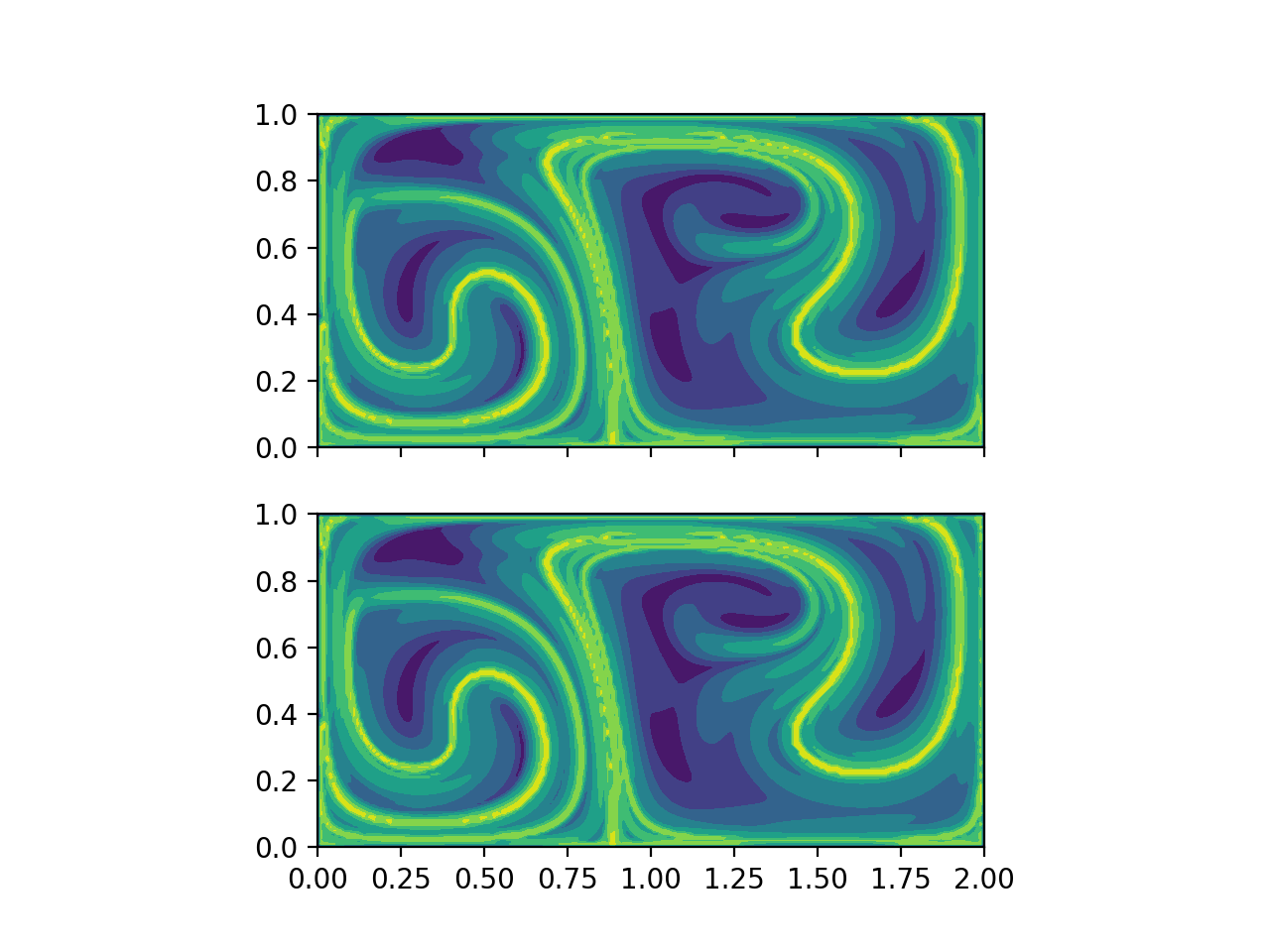
Plot FTLE from different flowmap methods

Plot FTLE from standard flowmap method and composition flowmap method. They are qualitatively indistinguishable.

i = 5
fig, axs = plt.subplots(nrows=2, ncols=1, sharex=True, dpi=200)
axs[0].contourf(x, y, ftle[i, :, :].T)
axs[1].contourf(x, y, ftlec[i, :, :].T)
axs[0].set_aspect("equal")
axs[1].set_aspect("equal")

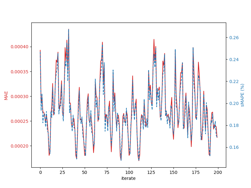
Error plots

Compute and plot error between FTLE from standard flowmap method and flowmap composition. Standard flowmap FTLE is assumed to be true value.

# mean absolute error
def MAE(true, est):
    """
    Compute mean absolute error.

    Parameters
    ----------
    true : np.ndarray
        true value.
    est : np.ndarray
        estimated value.

    Returns
    -------
    float
        mean absolute error.

    """
    n = true.size
    return np.sum(np.abs(true - est)) / n


# symmetric mean absolute percentage error
def sMAPE(true, est):
    """
    Compute symmetric mean absolute percentage error. In this form,
    true and est are assumed to be strictly positive.

    Parameters
    ----------
    true : np.ndarray
        true value.
    est : np.ndarray
        estimated value.

    Returns
    -------
    float
        symmetric mean absolute percentage error.

    """
    n = true.size
    return np.sum(np.divide(abs(true - est), true + est)) * (200 / n)


mae = np.zeros(n, np.float64)
smape = np.zeros(n, np.float64)
for k in range(n):
    f = ftle[k, :, :]
    f = f[f > 0]
    fc = ftlec[k, :, :]
    fc = fc[fc > 0]
    mae[k] = MAE(f, fc)
    smape[k] = sMAPE(f, fc)

fig, ax1 = plt.subplots(figsize=(8, 6))

color = "tab:red"
ax1.set_xlabel("iterate")
ax1.set_ylabel("MAE", color=color)
ax1.plot(mae, color=color)
ax1.tick_params(axis="y", labelcolor=color)

ax2 = ax1.twinx()

color = "tab:blue"
ax2.set_ylabel("sMAPE (%)", color=color)
ax2.plot(smape, "--", color=color)
ax2.tick_params(axis="y", labelcolor=color)