Quasi-geostrophic time series

Compare run times for different flowmap methods for the QGE.

# Author: ajarvis
# Data: We thank Changhong Mou and Traian Iliescu for providing us with this dataset
#       and allowing it to be used here.
# Hardware: Intel(R) Core(TM) i7-3770K CPU @ 3.50GHz, Cores = 4, Threads = 8

import numpy as np
from interpolation.splines import UCGrid
from numbacs.integration import (
    flowmap_grid_2D,
    flowmap_composition_initial,
    flowmap_composition_step,
)
from numbacs.flows import get_interp_arrays_2D, get_flow_2D
from numbacs.diagnostics import ftle_grid_2D
import matplotlib.pyplot as plt
import time
from math import copysign
import numba
from numba import njit, prange

Get flow data

Load velocity data, set up domain, set the integration span and direction, create interpolant of velocity data and retrieve necessary arrays.

# load in qge velocity data
u = np.load("../data/qge/qge_u.npy")
v = np.load("../data/qge/qge_v.npy")

# set up domain
nt, nx, ny = u.shape
x = np.linspace(0, 1, nx)
y = np.linspace(0, 2, ny)
t = np.linspace(0, 1, nt)
dx = x[1] - x[0]
dy = y[1] - y[0]

# set integration span and integration direction
t0 = 0.0
T = 0.1
params = np.array([copysign(1, T)])  # important this is an array of type float

# get interpolant arrays of velocity field
grid_vel, C_eval_u, C_eval_v = get_interp_arrays_2D(t, x, y, u, v)

# get flow to be integrated
funcptr = get_flow_2D(grid_vel, C_eval_u, C_eval_v, extrap_mode="linear")

Warm-up

Run flowmap_grid_2D and ftle_grid_2D so warm-up time is not included in comparison.

wfm = time.perf_counter()
flowmap_wu = flowmap_grid_2D(funcptr, t0, T, x, y, params)
wu_fm = time.perf_counter() - wfm
print(f"Flowmap with warm-up took {wu_fm:.5f} seconds")

wf = time.perf_counter()
ftle_wu = ftle_grid_2D(flowmap_wu, T, dx, dy)
wu_f = time.perf_counter() - wf
print(f"FTLE with warm-up took {wu_f:.5f} seconds")

Flowmap with warm-up took 2.32413 seconds
FTLE with warm-up took 0.02529 seconds

Set flowmap composition parameters

h = 0.005
grid = UCGrid((x[0], x[-1], nx), (y[0], y[-1], ny))
n = 50
tspan = np.arange(t0, t0 + n * h, h)

Flowmap composition

Perform flowmap composition over tspan and compute time series of FTLE.

ftlec = np.zeros((n, nx, ny), np.float64)
ctt = 0
c0s = time.perf_counter()
flowmap0, flowmaps, nT = flowmap_composition_initial(funcptr, t0, T, h, x, y, grid, params)
c0f = time.perf_counter()
c0 = c0f - c0s
ctt += c0

ftt = 0
f0s = time.perf_counter()
ftlec[0, :, :] = ftle_grid_2D(flowmap0, T, dx, dy)
f0f = time.perf_counter()
f0 = f0s - f0f
ftt += f0
for k in range(1, n):
    t0 = tspan[k] + T - h
    cks = time.perf_counter()
    flowmap_k, flowmaps = flowmap_composition_step(flowmaps, funcptr, t0, h, nT, x, y, grid, params)
    ckf = time.perf_counter()
    ctt += ckf - cks

    fks = time.perf_counter()
    ftlec[k, :, :] = ftle_grid_2D(flowmap_k, T, dx, dy)
    fkf = time.perf_counter()
    ftt += fkf - fks

print(f"Flowmap and FTLE computation (composed flowmap) took {ctt + ftt:.5f} seconds")
print(f"Average time for flowmap and FTLE was {(ctt + ftt) / n:.5f} seconds")
print(f"Average time for flowmap was {ctt / n:.5f} seconds")
print(f"Average time for FTLE was {ftt / n:.5f} seconds")
print(f"\nInitial flowmap integration and composition took {c0:.5f} seconds")
print(f"Average time for flowmap composition was {(ctt - c0) / (n - 1):.5f} seconds")

cfmtt = ctt + ftt
cfmat = ((ctt - c0) + (ftt - f0)) / (n - 1)

Flowmap and FTLE computation (composed flowmap) took 18.96519 seconds
Average time for flowmap and FTLE was 0.37930 seconds
Average time for flowmap was 0.35007 seconds
Average time for FTLE was 0.02924 seconds

Initial flowmap integration and composition took 3.80278 seconds
Average time for flowmap composition was 0.27960 seconds

Standard flowmap

Compute flowmap over tspan using a simple loop and the flowmap_grid_2D function, compute time series of FTLE. In this case, parallelization is performed over the spatial domain within the functions flowmap_grid_2D and ftle_grid_2D.

# set counter for total time and preallocate ftle
tt = 0
ftle = np.zeros((n, nx, ny), np.float64)
ftt = 0
# loop over initial times, compute flowmap and ftle
for k in range(n):
    t0 = tspan[k]
    ks = time.perf_counter()
    flowmap = flowmap_grid_2D(funcptr, t0, T, x, y, params)
    kf = time.perf_counter()
    kt = kf - ks
    tt += kt

    fks = time.perf_counter()
    ftle[k, :, :] = ftle_grid_2D(flowmap, T, dx, dy)
    fkf = time.perf_counter()
    ftt += fkf - fks

print(f"Flowmap and FTLE computation (parallel in space) took  {tt + ftt:.5f}")
print(f"Average time for flowmap and FTLE was {(tt + ftt) / n:.5f} seconds")
print(f"Average time for flowmap was {tt / n:.5f} seconds")
print(f"Average time for FTLE was {ftt / n:.5f} seconds")

fmtt = tt + ftt
fmat = (tt + ftt) / n

Flowmap and FTLE computation (parallel in space) took  121.41916
Average time for flowmap and FTLE was 2.42838 seconds
Average time for flowmap was 2.39646 seconds
Average time for FTLE was 0.03192 seconds

Parallelization over time

Alternatively, parallelization can be performed over time by creating a simple function as shown below. This provides a moderate speed up (depending on the hardware being used and the length of tspan). Functions like this can be created for any diagnostic or extraction method.

# function which moves the parallel load to the time domain
# instead of spatial domain
@njit(parallel=True)
def ftle_tspan(funcptr, tspan, T, x, y, params):
    """
    Function to compute time series of ftle fields in parallel.

    Parameters
    ----------
    funcptr : int
        pointer to C callback.
    tspan : np.ndarray, shape = (nt,)
        array containing times at which to compute ftle.
    T : float
        integration time.
    x : np.ndarray, shape = (nx,)
        array containing x-values.
    y : np.ndarray, shape = (ny,)
        array containing y-values.
    params : np.ndarray, shape = (nprms,)
        array of parameters to be passed to the ode function defined by funcptr.

    Returns
    -------
    ftle : np.ndarray, shape = (nt,nx,ny)
        array containing ftle fields for each t0 in tspan.

    """
    nx = len(x)
    ny = len(y)
    dx = x[1] - x[0]
    dy = y[1] - y[0]
    nt = len(tspan)
    ftle = np.zeros((nt, nx, ny), numba.float64)
    for k in prange(nt):
        t0 = tspan[k]
        flowmap = flowmap_grid_2D(funcptr, t0, T, x, y, params)
        ftle[k, :, :] = ftle_grid_2D(flowmap, T, dx, dy)

    return ftle


pt0 = time.perf_counter()
ftlep = ftle_tspan(funcptr, tspan, T, x, y, params)
ptt = time.perf_counter() - pt0
print(f"Flowmap and FTLE computation (parallel in time) took {ptt:.5f} seconds")
print(f"Average time for flowmap and FTLE was {ptt / n:.5f} seconds")

pfmtt = ptt
pfmat = ptt / n

Flowmap and FTLE computation (parallel in time) took 116.71094 seconds
Average time for flowmap and FTLE was 2.33422 seconds

Compare timings

Compare timings and quantify speedup

d1 = 5
d2 = 2
data = [
    [round(fmtt, d1), round(fmtt / fmtt, d2), round(fmat / fmat, d2)],
    [round(pfmtt, d1), round(fmtt / pfmtt, d2), round(fmat / pfmat, d2)],
    [round(cfmtt, d1), round(fmtt / cfmtt, d2), round(fmat / cfmat, d2)],
]

times = [f"total time (n={n})", "x speedup", "x speedup (per step)"]
methods = ["standard", "parallel time", "composition"]

format_row = "{:>25}" * (len(data[0]) + 1)

print(format_row.format("", *times))

for name, vals in zip(methods, data):
    print(format_row.format(name, *vals))

                     total time (n=50)                x speedup     x speedup (per step)
     standard                121.41916                      1.0                      1.0
parallel time                116.71094                     1.04                     1.04
  composition                 18.96519                      6.4                     7.83

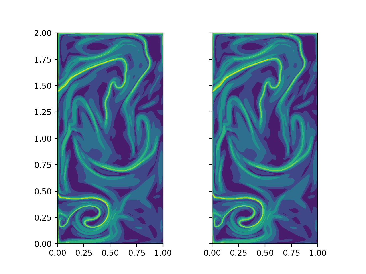
Plot FTLE from different flowmap methods

Plot FTLE from standard flowmap method and composition flowmap method. They are qualitatively indistinguishable.

i = 5
fig, axs = plt.subplots(nrows=1, ncols=2, sharey=True, dpi=200)
axs[0].contourf(x, y, ftle[i, :, :].T)
axs[1].contourf(x, y, ftlec[i, :, :].T)
axs[0].set_aspect("equal")
axs[1].set_aspect("equal")

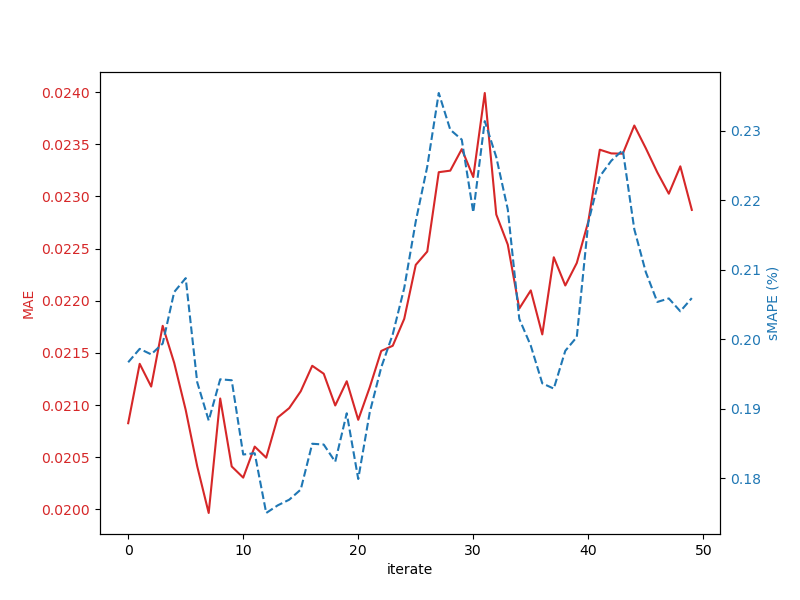
Error plots

Compute and plot error between FTLE from standard flowmap method and flowmap composition. Standard flowmap FTLE is assumed to be true value.

# mean absolute error
def MAE(true, est):
    """
    Compute mean absolute error.

    Parameters
    ----------
    true : np.ndarray
        true value.
    est : np.ndarray
        estimated value.

    Returns
    -------
    float
        mean absolute error.

    """
    n = true.size
    return np.sum(np.abs(true - est)) / n


# symmetric mean absolute percentage error
def sMAPE(true, est):
    """
    Compute symmetric mean absolute percentage error. In this form,
    true and est are assumed to be strictly positive.

    Parameters
    ----------
    true : np.ndarray
        true value.
    est : np.ndarray
        estimated value.

    Returns
    -------
    float
        symmetric mean absolute percentage error.

    """
    n = true.size
    return np.sum(np.divide(abs(true - est), true + est)) * (200 / n)


mae = np.zeros(n, np.float64)
smape = np.zeros(n, np.float64)
for k in range(n):
    f = ftle[k, :, :]
    zmask = f > 0
    f = f[zmask]
    fc = ftlec[k, :, :]
    fc = fc[zmask]
    mae[k] = MAE(f, fc)
    smape[k] = sMAPE(f, fc)

fig, ax1 = plt.subplots(figsize=(8, 6))

color = "tab:red"
ax1.set_xlabel("iterate")
ax1.set_ylabel("MAE", color=color)
ax1.plot(mae, color=color)
ax1.tick_params(axis="y", labelcolor=color)

ax2 = ax1.twinx()

color = "tab:blue"
ax2.set_ylabel("sMAPE (%)", color=color)
ax2.plot(smape, "--", color=color)
ax2.tick_params(axis="y", labelcolor=color)